Project 2
Ifeoma Ojialor 10/16/2020
Introduction
In this project, we will use a bike-sharing dataset to create machine
learning models. Before moving forward, I will briefly explain the
bike-sharing system and how it works. A bike-sharing system is a service
in which users can rent/use bicycles on a short term basis for a fee.
The goal of these programs is to provide affordable access to bicycles
for short distance trips as opposed to walking or taking public
transportation. Imagine how many people use these systems on a given
day, the numbers can vary greatly based on some elements. The goal of
this project is to build a predictive model to find out the number of
people that use these bikes in a given time period using available
information about that time/day. This in turn, can help businesses that
oversee this systems to manage them in a cost efficient manner.
We will be using the bike-sharing dataset from the UCL Machine Learning
Repository. We will use the regression and boosted tree method to model
the response variable cnt.
Exploratory Data Analysis
First we will read in the data using a relative path.
#read in data and filter to desired weekday
day1 <- read.csv("Bike-Sharing-Dataset/day.csv")
head(day1,5)
##   instant     dteday season yr mnth holiday weekday workingday weathersit
## 1       1 2011-01-01      1  0    1       0       6          0          2
## 2       2 2011-01-02      1  0    1       0       0          0          2
## 3       3 2011-01-03      1  0    1       0       1          1          1
## 4       4 2011-01-04      1  0    1       0       2          1          1
## 5       5 2011-01-05      1  0    1       0       3          1          1
##       temp    atemp      hum windspeed casual registered  cnt
## 1 0.344167 0.363625 0.805833  0.160446    331        654  985
## 2 0.363478 0.353739 0.696087  0.248539    131        670  801
## 3 0.196364 0.189405 0.437273  0.248309    120       1229 1349
## 4 0.200000 0.212122 0.590435  0.160296    108       1454 1562
## 5 0.226957 0.229270 0.436957  0.186900     82       1518 1600
Next, we will remove the casual and registered variables since the
cnt variable is a combination of both.
day1 <- select(day1, -casual, -registered)
day1$weekday <- as.factor(day1$weekday)
levels(day1$weekday) <- c("Sunday", "Monday", "Tuesday", "Wednesday", "Thursday", "Friday", "Saturday")
day <- filter(day1, weekday == params$days)

#Check for missing values
miss <- data.frame(apply(day,2,function(x){sum(is.na(x))}))
names(miss)[1] <- "missing"
miss
##            missing
## instant          0
## dteday           0
## season           0
## yr               0
## mnth             0
## holiday          0
## weekday          0
## workingday       0
## weathersit       0
## temp             0
## atemp            0
## hum              0
## windspeed        0
## cnt              0
There are no missing values in the dataset, so we can continue with our analysis.
#Change the variables into their appropriate format.
day$season <- as.factor(day$season)
day$weathersit <- as.factor(day$weathersit)
day$holiday <- as.factor(day$holiday)
day$workingday <- as.factor(day$workingday)
day$yr <- as.factor(day$yr)
day$mnth <- as.factor(day$mnth)

levels(day$season) <- c("winter", "spring", "summer", "fall")
levels(day$yr) <- c("2011", "2012")
str(day)
## 'data.frame':    104 obs. of  14 variables:
##  $ instant   : int  5 12 19 26 33 40 47 54 61 68 ...
##  $ dteday    : chr  "2011-01-05" "2011-01-12" "2011-01-19" "2011-01-26" ...
##  $ season    : Factor w/ 4 levels "winter","spring",..: 1 1 1 1 1 1 1 1 1 1 ...
##  $ yr        : Factor w/ 2 levels "2011","2012": 1 1 1 1 1 1 1 1 1 1 ...
##  $ mnth      : Factor w/ 12 levels "1","2","3","4",..: 1 1 1 1 2 2 2 2 3 3 ...
##  $ holiday   : Factor w/ 2 levels "0","1": 1 1 1 1 1 1 1 1 1 1 ...
##  $ weekday   : Factor w/ 7 levels "Sunday","Monday",..: 4 4 4 4 4 4 4 4 4 4 ...
##  $ workingday: Factor w/ 2 levels "0","1": 2 2 2 2 2 2 2 2 2 2 ...
##  $ weathersit: Factor w/ 3 levels "1","2","3": 1 1 2 3 2 2 1 1 1 2 ...
##  $ temp      : num  0.227 0.173 0.292 0.217 0.26 ...
##  $ atemp     : num  0.229 0.16 0.298 0.204 0.254 ...
##  $ hum       : num  0.437 0.6 0.742 0.863 0.775 ...
##  $ windspeed : num  0.187 0.305 0.208 0.294 0.264 ...
##  $ cnt       : int  1600 1162 1650 506 1526 1605 2115 1917 2134 1891 ...
Univariate Analysis
The cnt is the response variable, so we’ll use a histogram to get a
visual understanding of the variable.
ggplot(day, aes(x = cnt)) + theme_bw() + geom_histogram(aes(y =..density..), color = "black", fill = "white", binwidth = 1000) + geom_density(alpha = 0.2, fill = "blue") + labs(title = "Count Density", x = "Count", y = "Density")
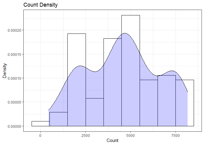
summary(day$cnt)
##    Min. 1st Qu.  Median    Mean 3rd Qu.    Max.
##     441    2653    4642    4549    6176    8173
From the histogram and summary statistics output, it is pretty evident that the count of total rental bikes are in the sub 5000 range. We will investigate if there is a relationship between the response variable and other relevant predictor variables in the next section. Lets look at the other variables individually.
#visualize numeric predictor variables using a histogram
p1 <- ggplot(day) + geom_histogram(aes(x = temp), fill = "red", binwidth = 0.03)
p2 <- ggplot(day) + geom_histogram(aes(x = atemp), fill = "red", binwidth = 0.03)
p3 <- ggplot(day) + geom_histogram(aes(x = hum), fill = "red", binwidth = 0.025)
p4 <- ggplot(day) + geom_histogram(aes(x = windspeed), fill = "red", binwidth = 0.03)
gridExtra::grid.arrange(p1,p2,p3,p4, nrow = 2)
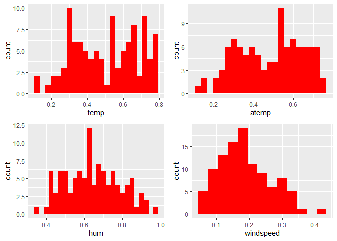
Observations:
* No clear cut pattern in tempand atemp.
-
humappears to be skewed to the left when the dataset is not filtered to a specific weekday. -
windspeedappears to be skewed(right). This variable should be transformed to curb its skewness. -
The distribution of
tempandatemplooks very similar. We should think about taking out one of the variables.
#visualize categorical predictor variables
h1 <- ggplot(day) + geom_bar(aes(x = season),fill = "pink")
h2 <- ggplot(day) + geom_bar(aes(x = yr),fill = "pink")
h3 <- ggplot(day) + geom_bar(aes(x = holiday),fill = "pink")
h4 <- ggplot(day) + geom_bar(aes(x = workingday),fill = "pink")
h5 <- ggplot(day) + geom_bar(aes(x = mnth),fill = "pink")
h6 <- ggplot(day) + geom_bar(aes(x = weathersit),fill = "pink")
gridExtra::grid.arrange(h1,h2,h3,h4,h5,h6, nrow = 3)
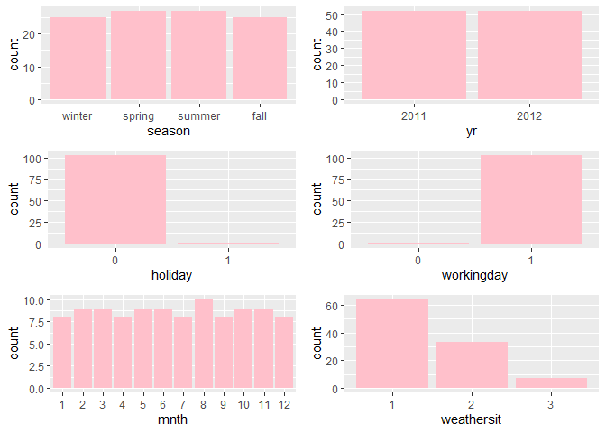
Observations:
* The variation between the four seasons is little to none.
-
About the same number of people rode bikes in 2011 and 2012.
-
Many people rode bikes on days that are not holidays.
-
Most people used the bike-sharing system on days that were neither weekends nor holidays.
-
Most people used the bike sharing system on days with clear weather.
Bi-variate Analysis
In this section, we will explore the predictor variables with respect to the response variable. The objective is to discover hidden relationships between the independent and response variables and use those findings in the model building process.
# First, we will explore the relationship between the target and numerical variables.
p1 <- ggplot(day) +geom_point(aes(x = temp, y = cnt), colour = "violet") + labs(title = "Normalized Temperature vs Total Rental Bikes")
p2 <- ggplot(day) +geom_point(aes(x = atemp, y = cnt), colour = "#FF99CC") +labs(title = "Normalized Feeling Temperature vs Total Rental Bikes")
p3 <- ggplot(day) +geom_point(aes(x = hum, y = cnt), colour = "pink") + labs(title = "Normalized Humidity vs Total rental Bikes")
p4 <- ggplot(day) +geom_point(aes(x = windspeed, y = cnt), colour = "#FF66CC") +labs(title= "Normalized Windspeed vs Total rental Bikes")
gridExtra::grid.arrange(p1, p2, p3, p4, nrow = 2)
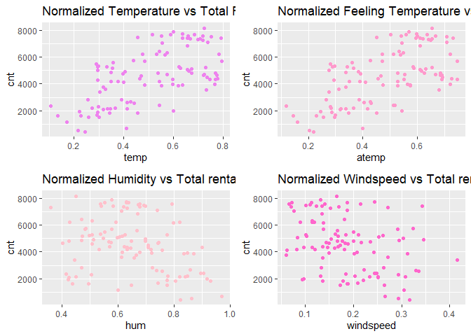
Observations:
* There appears to be a positive linear relationship between cnt ,
temp, and atemp.
- There is also a weak relationship between
cnt,hum, andwindspeed.
# Now we'll visualize the relationship between the target and categorical variables.
# Instead of using a boxplot, I will use a violin plot which is the blend of both a boxplot and density plot
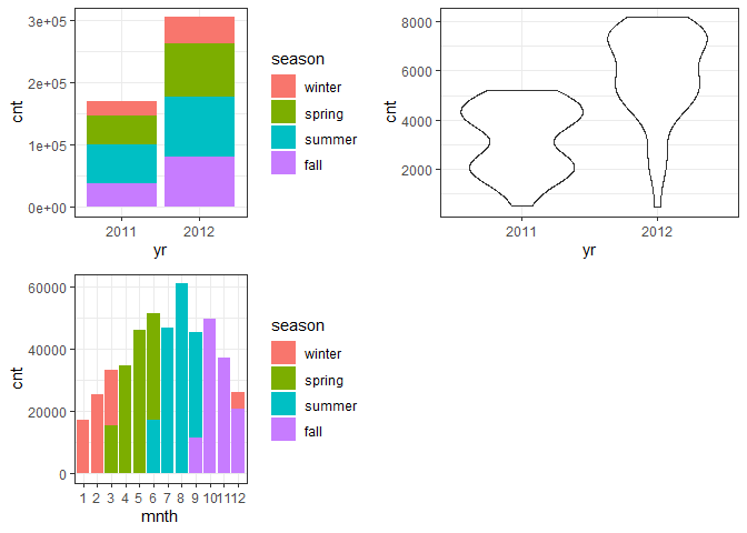
g1 <- ggplot(day) + geom_col(aes(x = yr, y = cnt, fill = season))+theme_bw()
g2 <- ggplot(day) + geom_violin(aes(x = yr, y = cnt))+theme_bw()
g3 <- ggplot(day) + geom_col(aes(x = mnth, y = cnt, fill = season))+theme_bw()
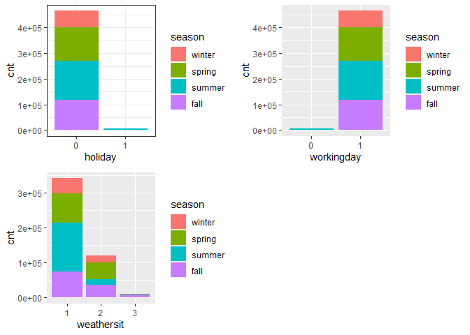
g4 <- ggplot(day) + geom_col(aes(x = holiday, y = cnt, fill = season)) + theme_bw()
g6 <- ggplot(day) + geom_col(aes(x = workingday, y = cnt, fill = season))
g7 <- ggplot(day) + geom_col(aes(x = weathersit, y = cnt, fill = season))
gridExtra::grid.arrange(g1, g2, g3, nrow = 2)
gridExtra::grid.arrange(g4, g6, g7, nrow = 2)
 Observations:
* The total bike rental count is higher in 2012 than 2011.
-
During workingday, the bike rental counts quite the highest compared to during no working day for different seasons.
-
During clear,partly cloudy weather, the bike rental count is highest and the second highest is during mist cloudy weather and followed by third highest during light snow and light rain weather.
-
The highest bike rental count was during the summer and lowest in the winter.
Correlation Matrix
Correlation matrix helps us to understand the linear relationship between variables.
day_c <- day[ , c(10:14)]
round(cor(day_c), 2)
##            temp atemp   hum windspeed   cnt
## temp       1.00  1.00  0.02     -0.32  0.62
## atemp      1.00  1.00  0.04     -0.35  0.63
## hum        0.02  0.04  1.00     -0.14 -0.31
## windspeed -0.32 -0.35 -0.14      1.00 -0.35
## cnt        0.62  0.63 -0.31     -0.35  1.00
From the above matrix, we can see that temp and atemp are highly
correlated. So we only need to include one of these variables in the
model to prevent multicollinearity. We will also transform the humidity
and windspeed variable.
day <- mutate(day, log_hum = log(day$hum+1))
day <- mutate(day, log_ws = log(day$windspeed + 1))

#Remove irrelevant variables
day <- select(day, -weekday,-holiday,-workingday,-dteday,-temp, -instant)
Model Building
First we split the data into train and test sets.
set.seed(23)
dayIndex<- createDataPartition(day$cnt, p = 0.7, list=FALSE)
dayTrain <- day[dayIndex, ]
dayTest <- day[-dayIndex, ]

# Build a tree-based model using loocv;
fitTree <- train(cnt~ ., data = dayTrain, method = "rpart",
              preProcess = c("center", "scale"),
              trControl = trainControl(method = "loocv", number = 10), tuneGrid = data.frame(cp = 0.01:0.10))
## Warning in nominalTrainWorkflow(x = x, y = y, wts = weights, info =
## trainInfo, : There were missing values in resampled performance measures.
# Build a boosted tree model using cv
fitBoost <- train(cnt~., data = dayTrain, method = "gbm",
              preProcess = c("center", "scale"),
              trControl = trainControl(method = "cv", number = 10),
              tuneGrid = expand.grid(n.trees=c(10,20,50,100,500,1000),shrinkage=c(0.01,0.05,0.1,0.5),n.minobsinnode =c(3,5,10),interaction.depth=c(1,5,10)))

# Adding a linear regression model part 2!
FitLinear <- train(cnt~ atemp + mnth*season, data = dayTrain, method = "lm", trControl = trainControl(method = "cv", number = 10))
## Warning in predict.lm(modelFit, newdata): prediction from a rank-deficient
## fit may be misleading

## Warning in predict.lm(modelFit, newdata): prediction from a rank-deficient
## fit may be misleading

## Warning in predict.lm(modelFit, newdata): prediction from a rank-deficient
## fit may be misleading

## Warning in predict.lm(modelFit, newdata): prediction from a rank-deficient
## fit may be misleading

## Warning in predict.lm(modelFit, newdata): prediction from a rank-deficient
## fit may be misleading

## Warning in predict.lm(modelFit, newdata): prediction from a rank-deficient
## fit may be misleading

## Warning in predict.lm(modelFit, newdata): prediction from a rank-deficient
## fit may be misleading

## Warning in predict.lm(modelFit, newdata): prediction from a rank-deficient
## fit may be misleading

## Warning in predict.lm(modelFit, newdata): prediction from a rank-deficient
## fit may be misleading

## Warning in predict.lm(modelFit, newdata): prediction from a rank-deficient
## fit may be misleading
# Display information from the tree fit
fitTree$results
##     cp     RMSE Rsquared      MAE   RMSESD RsquaredSD    MAESD
## 1 0.01 1009.592      NaN 1009.592 841.3955         NA 841.3955
# Display information from the boost fit
fitBoost$results
##     shrinkage interaction.depth n.minobsinnode n.trees      RMSE
## 1        0.01                 1              3      10 2003.5110
## 7        0.01                 1              5      10 2005.0402
## 13       0.01                 1             10      10 2002.9053
## 55       0.05                 1              3      10 1761.4426
## 61       0.05                 1              5      10 1731.6272
## 67       0.05                 1             10      10 1762.6538
## 109      0.10                 1              3      10 1529.3440
## 115      0.10                 1              5      10 1535.8142
## 121      0.10                 1             10      10 1503.9509
## 163      0.50                 1              3      10  840.3357
## 169      0.50                 1              5      10  971.6787
## 175      0.50                 1             10      10  961.2686
## 19       0.01                 5              3      10 1930.2847
## 25       0.01                 5              5      10 1937.1986
## 31       0.01                 5             10      10 1981.2736
## 73       0.05                 5              3      10 1509.4906
## 79       0.05                 5              5      10 1523.1294
## 85       0.05                 5             10      10 1668.4364
## 127      0.10                 5              3      10 1149.7461
## 133      0.10                 5              5      10 1198.5117
## 139      0.10                 5             10      10 1411.2833
## 181      0.50                 5              3      10  950.6159
## 187      0.50                 5              5      10  872.6785
## 193      0.50                 5             10      10  979.4999
## 37       0.01                10              3      10 1926.1261
## 43       0.01                10              5      10 1937.3569
## 49       0.01                10             10      10 1982.5054
## 91       0.05                10              3      10 1481.9732
## 97       0.05                10              5      10 1520.8688
## 103      0.05                10             10      10 1693.0784
## 145      0.10                10              3      10 1128.3697
## 151      0.10                10              5      10 1174.7133
## 157      0.10                10             10      10 1437.0837
## 199      0.50                10              3      10  930.5235
## 205      0.50                10              5      10  891.1722
## 211      0.50                10             10      10 1015.8159
## 2        0.01                 1              3      20 1939.9855
## 8        0.01                 1              5      20 1937.5667
## 14       0.01                 1             10      20 1935.8531
## 56       0.05                 1              3      20 1522.5367
## 62       0.05                 1              5      20 1504.9166
## 68       0.05                 1             10      20 1502.4161
## 110      0.10                 1              3      20 1166.6471
## 116      0.10                 1              5      20 1163.3336
## 122      0.10                 1             10      20 1160.8975
## 164      0.50                 1              3      20  844.3312
## 170      0.50                 1              5      20  910.0425
## 176      0.50                 1             10      20  895.7659
## 20       0.01                 5              3      20 1810.2379
## 26       0.01                 5              5      20 1817.4687
## 32       0.01                 5             10      20 1902.2482
## 74       0.05                 5              3      20 1166.1182
## 80       0.05                 5              5      20 1214.7805
## 86       0.05                 5             10      20 1399.2135
## 128      0.10                 5              3      20  869.7473
## 134      0.10                 5              5      20  920.9463
## 140      0.10                 5             10      20 1082.7860
## 182      0.50                 5              3      20 1011.1812
## 188      0.50                 5              5      20  844.0630
## 194      0.50                 5             10      20 1015.8730
## 38       0.01                10              3      20 1796.8704
## 44       0.01                10              5      20 1817.1011
## 50       0.01                10             10      20 1901.7880
## 92       0.05                10              3      20 1161.4540
## 98       0.05                10              5      20 1213.8890
## 104      0.05                10             10      20 1427.2983
## 146      0.10                10              3      20  861.1810
## 152      0.10                10              5      20  877.4350
## 158      0.10                10             10      20 1104.1391
## 200      0.50                10              3      20  956.4472
## 206      0.50                10              5      20  865.4356
## 212      0.50                10             10      20  999.4744
## 3        0.01                 1              3      50 1757.7308
## 9        0.01                 1              5      50 1758.3215
## 15       0.01                 1             10      50 1753.0252
## 57       0.05                 1              3      50 1067.8686
## 63       0.05                 1              5      50 1048.8467
## 69       0.05                 1             10      50 1094.3583
## 111      0.10                 1              3      50  832.4108
## 117      0.10                 1              5      50  814.7430
## 123      0.10                 1             10      50  916.3512
## 165      0.50                 1              3      50  866.5046
## 171      0.50                 1              5      50  909.5119
## 177      0.50                 1             10      50  889.0260
## 21       0.01                 5              3      50 1511.9527
## 27       0.01                 5              5      50 1536.1063
## 33       0.01                 5             10      50 1692.9896
## 75       0.05                 5              3      50  800.2739
## 81       0.05                 5              5      50  855.7534
## 87       0.05                 5             10      50  993.2033
## 129      0.10                 5              3      50  731.1433
## 135      0.10                 5              5      50  751.2279
## 141      0.10                 5             10      50  898.0954
## 183      0.50                 5              3      50  979.5400
## 189      0.50                 5              5      50  881.2239
## 195      0.50                 5             10      50  955.9519
## 39       0.01                10              3      50 1480.9279
## 45       0.01                10              5      50 1526.6101
## 51       0.01                10             10      50 1684.9244
## 93       0.05                10              3      50  832.8529
##      Rsquared       MAE   RMSESD RsquaredSD    MAESD
## 1   0.6768312 1640.3976 190.6386 0.17491152 169.9711
## 7   0.7568004 1641.2535 193.2893 0.18366014 171.1636
## 13  0.6896555 1638.9103 199.1170 0.17916020 172.8409
## 55  0.7145130 1461.0394 220.4091 0.16832275 199.0373
## 61  0.8061605 1418.6178 239.5044 0.15618442 213.5705
## 67  0.7428956 1463.3998 223.7200 0.10988157 197.1943
## 109 0.7931334 1270.3528 254.9077 0.14225827 218.5391
## 115 0.8143601 1265.4821 203.6620 0.11460952 173.3305
## 121 0.8182785 1248.6813 273.7063 0.11783854 236.0999
## 163 0.8979910  699.5439 191.2471 0.03207193 175.3628
## 169 0.8320873  822.2528 307.8882 0.10630992 242.5387
## 175 0.8370860  736.4121 231.5725 0.08189839 155.7015
## 19  0.8228225 1578.0487 194.2706 0.10499200 173.8053
## 25  0.8071988 1588.6924 197.6712 0.10663229 176.3829
## 31  0.7759350 1617.6537 193.6548 0.10938831 172.5538
## 73  0.8552803 1244.1635 214.0635 0.07958459 218.3713
## 79  0.8478814 1249.4145 223.9619 0.09643196 203.0674
## 85  0.8267608 1381.0214 213.1043 0.11637264 196.0549
## 127 0.8843493  965.3577 259.4657 0.06507090 193.9855
## 133 0.8504153 1014.3959 250.0548 0.09730283 186.5340
## 139 0.7998828 1179.8901 262.1009 0.11052028 213.3328
## 181 0.8376855  803.2571 392.6288 0.12931366 310.7862
## 187 0.8542920  693.9442 260.4394 0.09474814 232.1330
## 193 0.8308985  800.6531 202.9320 0.07836322 210.6601
## 37  0.8469114 1572.9844 194.5142 0.08403401 172.3453
## 43  0.7954160 1585.0434 199.5492 0.07572268 182.5217
## 49  0.7382241 1625.2817 194.9107 0.18894989 171.6316
## 91  0.8480249 1211.0767 240.4557 0.11675885 225.2132
## 97  0.8178433 1250.7015 236.2567 0.10072230 219.4936
## 103 0.7559111 1393.3797 214.6034 0.15022333 205.5787
## 145 0.8795814  939.1580 220.9623 0.07719079 167.4315
## 151 0.8536481  995.6709 235.4187 0.07771007 182.5564
## 157 0.8257081 1205.0283 251.6858 0.07017814 216.7241
## 199 0.8527535  737.7498 348.4425 0.11744550 313.1386
## 205 0.8677516  750.5687 297.4610 0.07768680 241.7777
## 211 0.8121407  831.5702 275.5315 0.09988316 213.2782
## 2   0.7024270 1591.8703 195.3415 0.18603207 170.5504
## 8   0.8142700 1586.5348 198.2240 0.16474637 171.8997
## 14  0.7300955 1587.0580 205.8460 0.15255345 177.7830
## 56  0.8138074 1257.9261 236.5598 0.12240405 214.4159
## 62  0.8299665 1244.4751 230.0424 0.10761126 198.6976
## 68  0.8056603 1265.2350 227.9769 0.08496789 207.2635
## 110 0.8617492  981.9384 249.0905 0.07736403 201.5355
## 116 0.8845213  971.4092 233.6265 0.06056838 200.4127
## 122 0.8600711  955.5374 302.6252 0.08573966 262.1850
## 164 0.8893411  690.1620 127.9824 0.02824014 118.5144
## 170 0.8592425  779.4757 288.8131 0.08808383 246.9755
## 176 0.8561145  711.6794 244.8984 0.07084019 166.3895
## 20  0.8454855 1480.2967 196.4207 0.09336042 179.6772
## 26  0.8268481 1495.2653 203.9529 0.10451680 179.7013
## 32  0.7970830 1556.6928 198.6538 0.10867321 174.5170
## 74  0.8963237  983.0424 231.0656 0.07103000 191.5959
## 80  0.8595657 1013.0649 250.1154 0.10002728 182.4885
## 86  0.8441118 1168.3494 235.9731 0.07977645 196.4387
## 128 0.9005912  714.2848 285.9100 0.07091487 222.6245
## 134 0.8794067  759.2921 222.8855 0.08284108 173.8122
## 140 0.8503541  904.4939 243.9210 0.08224399 176.3867
## 182 0.8217559  851.4916 349.7952 0.11403941 273.4058
## 188 0.8736124  670.4354 278.6924 0.08533908 223.0973
## 194 0.8205671  814.7426 244.2476 0.08558901 231.2785
## 38  0.8650567 1466.8147 202.2002 0.08747740 179.1584
## 44  0.8148047 1491.1152 202.4300 0.08903062 187.7594
## 50  0.7876522 1559.5416 202.0606 0.15243225 177.7333
## 92  0.8717934  965.7937 261.0813 0.08812103 186.6116
## 98  0.8447348 1028.4998 236.4171 0.09477882 182.9314
## 104 0.8108340 1184.6895 248.8937 0.11479312 205.1195
## 146 0.9079926  702.5789 239.7628 0.05782067 189.3858
## 152 0.8880401  733.3538 246.9468 0.07573568 210.1960
## 158 0.8518390  931.6540 284.7119 0.08219733 205.6038
## 200 0.8511996  763.0262 296.4789 0.10703528 248.0589
## 206 0.8733187  719.9630 316.1076 0.09349143 276.0815
## 212 0.8419374  809.3398 228.4034 0.08244704 185.9003
## 3   0.8173478 1443.3626 205.4431 0.13294971 183.6042
## 9   0.8177642 1445.2356 208.9971 0.12579882 184.6085
## 15  0.7968873 1441.2541 218.6593 0.14672920 191.3141
## 57  0.8780072  903.3225 283.5515 0.08921183 239.0104
## 63  0.8755931  879.0805 280.4916 0.07600625 223.6982
## 69  0.8538346  916.9428 260.4017 0.07740422 213.8083
## 111 0.8907918  679.9504 232.7498 0.05993877 188.9045
## 117 0.9004314  671.3753 257.8127 0.05373681 219.2017
## 123 0.8751056  744.5392 274.9282 0.06889871 213.3865
## 165 0.8874578  719.8713 174.0566 0.05039699 159.9228
## 171 0.8730721  747.8428 277.2274 0.08070312 233.6273
## 177 0.8697784  729.0075 290.3578 0.09713687 255.3234
## 21  0.8797787 1239.5450 209.2677 0.07684662 195.8877
## 27  0.8535605 1259.0808 236.4155 0.08976171 231.0629
## 33  0.8220612 1388.9204 222.5593 0.11840459 193.8980
## 75  0.9095261  650.0294 258.8369 0.06587914 213.1944
## 81  0.8950032  689.4073 273.5048 0.07429349 206.6245
## 87  0.8684406  829.0928 242.8930 0.06685082 188.5989
## 129 0.9184942  592.5636 290.9533 0.05546817 229.8863
## 135 0.9079020  614.5137 267.3046 0.06108018 212.3541
## 141 0.8634789  734.3107 257.1552 0.07433480 192.4943
## 183 0.8288907  843.0503 366.9173 0.12231758 314.6615
## 189 0.8525163  719.2765 268.2056 0.09458521 227.4911
## 195 0.8304633  777.6060 253.1319 0.10928750 207.9205
## 39  0.8844109 1210.8669 220.6354 0.08425407 212.1545
## 45  0.8535966 1253.8497 226.0283 0.08632102 221.1928
## 51  0.8280065 1379.9484 222.6424 0.10198675 207.5980
## 93  0.8968213  677.1692 284.8553 0.06448944 225.8926
##  [ reached 'max' / getOption("max.print") -- omitted 116 rows ]
# Display information from the linear model fit
FitLinear$results
##   intercept     RMSE  Rsquared      MAE   RMSESD RsquaredSD    MAESD
## 1      TRUE 1955.282 0.2960616 1738.632 522.6991  0.2832465 467.5813
Now, we make predictions on the test data sets using the best model fits. Then we compare RMSE to determine the best model.
predTree <- predict(fitTree, newdata = select(dayTest, -cnt))
postResample(predTree, dayTest$cnt)
##        RMSE    Rsquared         MAE
## 1014.583865    0.772907  785.967780
boostPred <- predict(fitBoost, newdata = select(dayTest, -cnt))
postResample(boostPred, dayTest$cnt)
##        RMSE    Rsquared         MAE
## 687.3093774   0.8859169 549.7823124
linearPred <- predict(FitLinear, newdata = select(dayTest, -cnt))
## Warning in predict.lm(modelFit, newdata): prediction from a rank-deficient
## fit may be misleading
postResample(linearPred, dayTest$cnt)
##         RMSE     Rsquared          MAE
## 1584.1860790    0.3526254 1397.2144755
When we compare the two models, the boosted tree model has lower RMSE values when applied on the test dataset. Hence, the boosted tree model is our final model and best model for interpreting the bike rental count on a daily basis.