Project 2
Ifeoma Ojialor 10/16/2020
Introduction
In this project, we will use a bike-sharing dataset to create machine
learning models. Before moving forward, I will briefly explain the
bike-sharing system and how it works. A bike-sharing system is a service
in which users can rent/use bicycles on a short term basis for a fee.
The goal of these programs is to provide affordable access to bicycles
for short distance trips as opposed to walking or taking public
transportation. Imagine how many people use these systems on a given
day, the numbers can vary greatly based on some elements. The goal of
this project is to build a predictive model to find out the number of
people that use these bikes in a given time period using available
information about that time/day. This in turn, can help businesses that
oversee this systems to manage them in a cost efficient manner.
We will be using the bike-sharing dataset from the UCL Machine Learning
Repository. We will use the regression and boosted tree method to model
the response variable cnt.
Exploratory Data Analysis
First we will read in the data using a relative path.
#read in data and filter to desired weekday
day1 <- read.csv("Bike-Sharing-Dataset/day.csv")
head(day1,5)
##   instant     dteday season yr mnth holiday weekday workingday weathersit
## 1       1 2011-01-01      1  0    1       0       6          0          2
## 2       2 2011-01-02      1  0    1       0       0          0          2
## 3       3 2011-01-03      1  0    1       0       1          1          1
## 4       4 2011-01-04      1  0    1       0       2          1          1
## 5       5 2011-01-05      1  0    1       0       3          1          1
##       temp    atemp      hum windspeed casual registered  cnt
## 1 0.344167 0.363625 0.805833  0.160446    331        654  985
## 2 0.363478 0.353739 0.696087  0.248539    131        670  801
## 3 0.196364 0.189405 0.437273  0.248309    120       1229 1349
## 4 0.200000 0.212122 0.590435  0.160296    108       1454 1562
## 5 0.226957 0.229270 0.436957  0.186900     82       1518 1600
Next, we will remove the casual and registered variables since the
cnt variable is a combination of both.
day1 <- select(day1, -casual, -registered)
day1$weekday <- as.factor(day1$weekday)
levels(day1$weekday) <- c("Sunday", "Monday", "Tuesday", "Wednesday", "Thursday", "Friday", "Saturday")
day <- filter(day1, weekday == params$days)

#Check for missing values
miss <- data.frame(apply(day,2,function(x){sum(is.na(x))}))
names(miss)[1] <- "missing"
miss
##            missing
## instant          0
## dteday           0
## season           0
## yr               0
## mnth             0
## holiday          0
## weekday          0
## workingday       0
## weathersit       0
## temp             0
## atemp            0
## hum              0
## windspeed        0
## cnt              0
There are no missing values in the dataset, so we can continue with our analysis.
#Change the variables into their appropriate format.
day$season <- as.factor(day$season)
day$weathersit <- as.factor(day$weathersit)
day$holiday <- as.factor(day$holiday)
day$workingday <- as.factor(day$workingday)
day$yr <- as.factor(day$yr)
day$mnth <- as.factor(day$mnth)

levels(day$season) <- c("winter", "spring", "summer", "fall")
levels(day$yr) <- c("2011", "2012")
str(day)
## 'data.frame':    104 obs. of  14 variables:
##  $ instant   : int  4 11 18 25 32 39 46 53 60 67 ...
##  $ dteday    : chr  "2011-01-04" "2011-01-11" "2011-01-18" "2011-01-25" ...
##  $ season    : Factor w/ 4 levels "winter","spring",..: 1 1 1 1 1 1 1 1 1 1 ...
##  $ yr        : Factor w/ 2 levels "2011","2012": 1 1 1 1 1 1 1 1 1 1 ...
##  $ mnth      : Factor w/ 12 levels "1","2","3","4",..: 1 1 1 1 2 2 2 2 3 3 ...
##  $ holiday   : Factor w/ 2 levels "0","1": 1 1 1 1 1 1 1 1 1 1 ...
##  $ weekday   : Factor w/ 7 levels "Sunday","Monday",..: 3 3 3 3 3 3 3 3 3 3 ...
##  $ workingday: Factor w/ 2 levels "0","1": 2 2 2 2 2 2 2 2 2 2 ...
##  $ weathersit: Factor w/ 3 levels "1","2","3": 1 2 2 2 2 1 1 1 1 1 ...
##  $ temp      : num  0.2 0.169 0.217 0.223 0.192 ...
##  $ atemp     : num  0.212 0.191 0.232 0.235 0.235 ...
##  $ hum       : num  0.59 0.686 0.862 0.617 0.83 ...
##  $ windspeed : num  0.1603 0.1221 0.1468 0.1298 0.0532 ...
##  $ cnt       : int  1562 1263 683 1985 1360 1530 1815 1450 1851 2133 ...
Univariate Analysis
The cnt is the response variable, so we’ll use a histogram to get a
visual understanding of the variable.
ggplot(day, aes(x = cnt)) + theme_bw() + geom_histogram(aes(y =..density..), color = "black", fill = "white", binwidth = 1000) + geom_density(alpha = 0.2, fill = "blue") + labs(title = "Count Density", x = "Count", y = "Density")
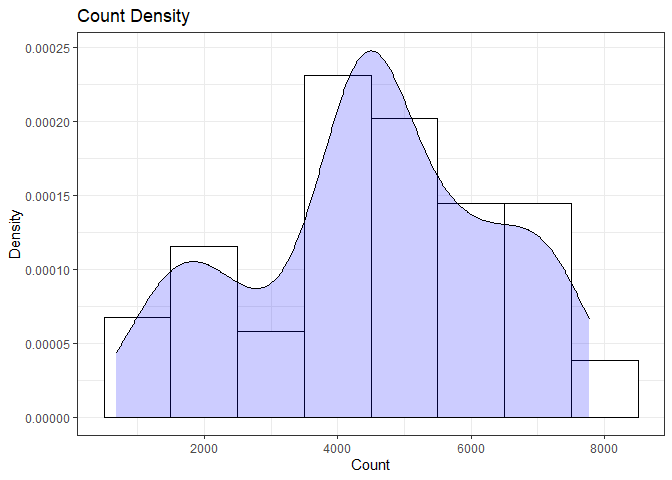
summary(day$cnt)
##    Min. 1st Qu.  Median    Mean 3rd Qu.    Max.
##     683    3579    4576    4511    5769    7767
From the histogram and summary statistics output, it is pretty evident that the count of total rental bikes are in the sub 5000 range. We will investigate if there is a relationship between the response variable and other relevant predictor variables in the next section. Lets look at the other variables individually.
#visualize numeric predictor variables using a histogram
p1 <- ggplot(day) + geom_histogram(aes(x = temp), fill = "red", binwidth = 0.03)
p2 <- ggplot(day) + geom_histogram(aes(x = atemp), fill = "red", binwidth = 0.03)
p3 <- ggplot(day) + geom_histogram(aes(x = hum), fill = "red", binwidth = 0.025)
p4 <- ggplot(day) + geom_histogram(aes(x = windspeed), fill = "red", binwidth = 0.03)
gridExtra::grid.arrange(p1,p2,p3,p4, nrow = 2)
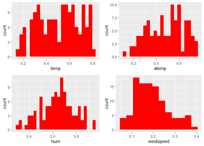
Observations:
* No clear cut pattern in tempand atemp.
-
humappears to be skewed to the left when the dataset is not filtered to a specific weekday. -
windspeedappears to be skewed(right). This variable should be transformed to curb its skewness. -
The distribution of
tempandatemplooks very similar. We should think about taking out one of the variables.
#visualize categorical predictor variables
h1 <- ggplot(day) + geom_bar(aes(x = season),fill = "pink")
h2 <- ggplot(day) + geom_bar(aes(x = yr),fill = "pink")
h3 <- ggplot(day) + geom_bar(aes(x = holiday),fill = "pink")
h4 <- ggplot(day) + geom_bar(aes(x = workingday),fill = "pink")
h5 <- ggplot(day) + geom_bar(aes(x = mnth),fill = "pink")
h6 <- ggplot(day) + geom_bar(aes(x = weathersit),fill = "pink")
gridExtra::grid.arrange(h1,h2,h3,h4,h5,h6, nrow = 3)
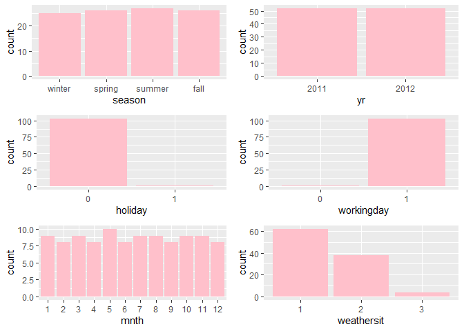
Observations:
* The variation between the four seasons is little to none.
-
About the same number of people rode bikes in 2011 and 2012.
-
Many people rode bikes on days that are not holidays.
-
Most people used the bike-sharing system on days that were neither weekends nor holidays.
-
Most people used the bike sharing system on days with clear weather.
Bi-variate Analysis
In this section, we will explore the predictor variables with respect to the response variable. The objective is to discover hidden relationships between the independent and response variables and use those findings in the model building process.
# First, we will explore the relationship between the target and numerical variables.
p1 <- ggplot(day) +geom_point(aes(x = temp, y = cnt), colour = "violet") + labs(title = "Normalized Temperature vs Total Rental Bikes")
p2 <- ggplot(day) +geom_point(aes(x = atemp, y = cnt), colour = "#FF99CC") +labs(title = "Normalized Feeling Temperature vs Total Rental Bikes")
p3 <- ggplot(day) +geom_point(aes(x = hum, y = cnt), colour = "pink") + labs(title = "Normalized Humidity vs Total rental Bikes")
p4 <- ggplot(day) +geom_point(aes(x = windspeed, y = cnt), colour = "#FF66CC") +labs(title= "Normalized Windspeed vs Total rental Bikes")
gridExtra::grid.arrange(p1, p2, p3, p4, nrow = 2)
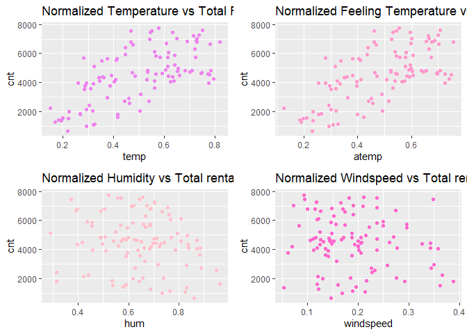
Observations:
* There appears to be a positive linear relationship between cnt ,
temp, and atemp.
- There is also a weak relationship between
cnt,hum, andwindspeed.
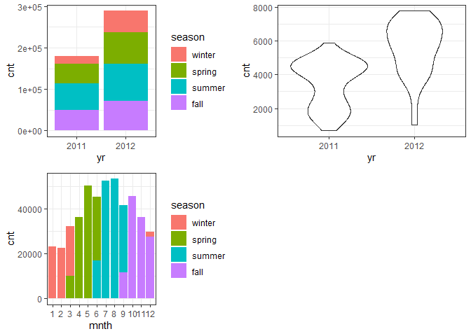
# Now we'll visualize the relationship between the target and categorical variables.
# Instead of using a boxplot, I will use a violin plot which is the blend of both a boxplot and density plot
g1 <- ggplot(day) + geom_col(aes(x = yr, y = cnt, fill = season))+theme_bw()
g2 <- ggplot(day) + geom_violin(aes(x = yr, y = cnt))+theme_bw()
g3 <- ggplot(day) + geom_col(aes(x = mnth, y = cnt, fill = season))+theme_bw()
g4 <- ggplot(day) + geom_col(aes(x = holiday, y = cnt, fill = season)) + theme_bw()
g6 <- ggplot(day) + geom_col(aes(x = workingday, y = cnt, fill = season))
g7 <- ggplot(day) + geom_col(aes(x = weathersit, y = cnt, fill = season))
gridExtra::grid.arrange(g1, g2, g3, nrow = 2)
gridExtra::grid.arrange(g4, g6, g7, nrow = 2)
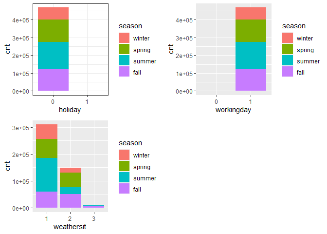 Observations:
* The total bike rental count is higher in 2012 than 2011.
-
During workingday, the bike rental counts quite the highest compared to during no working day for different seasons.
-
During clear,partly cloudy weather, the bike rental count is highest and the second highest is during mist cloudy weather and followed by third highest during light snow and light rain weather.
-
The highest bike rental count was during the summer and lowest in the winter.
Correlation Matrix
Correlation matrix helps us to understand the linear relationship between variables.
day_c <- day[ , c(10:14)]
round(cor(day_c), 2)
##            temp atemp   hum windspeed   cnt
## temp       1.00  1.00  0.11     -0.09  0.63
## atemp      1.00  1.00  0.12     -0.12  0.64
## hum        0.11  0.12  1.00     -0.10 -0.18
## windspeed -0.09 -0.12 -0.10      1.00 -0.15
## cnt        0.63  0.64 -0.18     -0.15  1.00
From the above matrix, we can see that temp and atemp are highly
correlated. So we only need to include one of these variables in the
model to prevent multicollinearity. We will also transform the humidity
and windspeed variable.
day <- mutate(day, log_hum = log(day$hum+1))
day <- mutate(day, log_ws = log(day$windspeed + 1))

#Remove irrelevant variables
day <- select(day, -weekday,-holiday,-workingday,-dteday,-temp, -instant)
Model Building
First we split the data into train and test sets.
set.seed(23)
dayIndex<- createDataPartition(day$cnt, p = 0.7, list=FALSE)
dayTrain <- day[dayIndex, ]
dayTest <- day[-dayIndex, ]

# Build a tree-based model using loocv;
fitTree <- train(cnt~ ., data = dayTrain, method = "rpart",
              preProcess = c("center", "scale"),
              trControl = trainControl(method = "loocv", number = 10), tuneGrid = data.frame(cp = 0.01:0.10))
## Warning in nominalTrainWorkflow(x = x, y = y, wts = weights, info =
## trainInfo, : There were missing values in resampled performance measures.
# Build a boosted tree model using cv
fitBoost <- train(cnt~., data = dayTrain, method = "gbm",
              preProcess = c("center", "scale"),
              trControl = trainControl(method = "cv", number = 10),
              tuneGrid = expand.grid(n.trees=c(10,20,50,100,500,1000),shrinkage=c(0.01,0.05,0.1,0.5),n.minobsinnode =c(3,5,10),interaction.depth=c(1,5,10)))

# Adding a linear regression model part 2!
FitLinear <- train(cnt~ atemp + mnth*season, data = dayTrain, method = "lm", trControl = trainControl(method = "cv", number = 10))
## Warning in predict.lm(modelFit, newdata): prediction from a rank-deficient
## fit may be misleading

## Warning in predict.lm(modelFit, newdata): prediction from a rank-deficient
## fit may be misleading

## Warning in predict.lm(modelFit, newdata): prediction from a rank-deficient
## fit may be misleading

## Warning in predict.lm(modelFit, newdata): prediction from a rank-deficient
## fit may be misleading

## Warning in predict.lm(modelFit, newdata): prediction from a rank-deficient
## fit may be misleading

## Warning in predict.lm(modelFit, newdata): prediction from a rank-deficient
## fit may be misleading

## Warning in predict.lm(modelFit, newdata): prediction from a rank-deficient
## fit may be misleading

## Warning in predict.lm(modelFit, newdata): prediction from a rank-deficient
## fit may be misleading

## Warning in predict.lm(modelFit, newdata): prediction from a rank-deficient
## fit may be misleading

## Warning in predict.lm(modelFit, newdata): prediction from a rank-deficient
## fit may be misleading
# Display information from the tree fit
fitTree$results
##     cp     RMSE Rsquared      MAE   RMSESD RsquaredSD    MAESD
## 1 0.01 823.6188      NaN 823.6188 658.3374         NA 658.3374
# Display information from the boost fit
fitBoost$results
##     shrinkage interaction.depth n.minobsinnode n.trees      RMSE
## 1        0.01                 1              3      10 1716.5908
## 7        0.01                 1              5      10 1717.0477
## 13       0.01                 1             10      10 1716.3381
## 55       0.05                 1              3      10 1530.0472
## 61       0.05                 1              5      10 1511.4705
## 67       0.05                 1             10      10 1512.9832
## 109      0.10                 1              3      10 1307.5567
## 115      0.10                 1              5      10 1340.6528
## 121      0.10                 1             10      10 1307.6531
## 163      0.50                 1              3      10  848.1331
## 169      0.50                 1              5      10  864.4649
## 175      0.50                 1             10      10  883.0600
## 19       0.01                 5              3      10 1655.3577
## 25       0.01                 5              5      10 1660.7433
## 31       0.01                 5             10      10 1694.9238
## 73       0.05                 5              3      10 1310.6083
## 79       0.05                 5              5      10 1338.8179
## 85       0.05                 5             10      10 1452.5004
## 127      0.10                 5              3      10 1093.6222
## 133      0.10                 5              5      10 1078.3550
## 139      0.10                 5             10      10 1251.7282
## 181      0.50                 5              3      10  887.4160
## 187      0.50                 5              5      10  853.1468
## 193      0.50                 5             10      10  937.2025
## 37       0.01                10              3      10 1655.3585
## 43       0.01                10              5      10 1666.9992
## 49       0.01                10             10      10 1693.4027
## 91       0.05                10              3      10 1323.5993
## 97       0.05                10              5      10 1355.0405
## 103      0.05                10             10      10 1453.2335
## 145      0.10                10              3      10 1071.1757
## 151      0.10                10              5      10 1100.2979
## 157      0.10                10             10      10 1231.7675
## 199      0.50                10              3      10  940.4929
## 205      0.50                10              5      10  736.3302
## 211      0.50                10             10      10  985.8810
## 2        0.01                 1              3      20 1665.9342
## 8        0.01                 1              5      20 1661.8524
## 14       0.01                 1             10      20 1662.3235
## 56       0.05                 1              3      20 1322.9027
## 62       0.05                 1              5      20 1332.0855
## 68       0.05                 1             10      20 1308.2128
## 110      0.10                 1              3      20 1100.2823
## 116      0.10                 1              5      20 1095.9149
## 122      0.10                 1             10      20 1120.3766
## 164      0.50                 1              3      20  749.2292
## 170      0.50                 1              5      20  801.4227
## 176      0.50                 1             10      20  816.5135
## 20       0.01                 5              3      20 1562.4757
## 26       0.01                 5              5      20 1564.3416
## 32       0.01                 5             10      20 1629.9705
## 74       0.05                 5              3      20 1075.5512
## 80       0.05                 5              5      20 1101.6318
## 86       0.05                 5             10      20 1249.3434
## 128      0.10                 5              3      20  861.0841
## 134      0.10                 5              5      20  859.0220
## 140      0.10                 5             10      20 1053.6645
## 182      0.50                 5              3      20  884.6596
## 188      0.50                 5              5      20  832.7330
## 194      0.50                 5             10      20  935.9977
## 38       0.01                10              3      20 1554.6247
## 44       0.01                10              5      20 1573.5106
## 50       0.01                10             10      20 1628.6780
## 92       0.05                10              3      20 1077.9416
## 98       0.05                10              5      20 1108.9181
## 104      0.05                10             10      20 1249.3974
## 146      0.10                10              3      20  858.6573
## 152      0.10                10              5      20  889.8509
## 158      0.10                10             10      20 1017.0416
## 200      0.50                10              3      20  928.5215
## 206      0.50                10              5      20  767.4830
## 212      0.50                10             10      20  924.7482
## 3        0.01                 1              3      50 1519.4490
## 9        0.01                 1              5      50 1513.4075
## 15       0.01                 1             10      50 1517.2969
## 57       0.05                 1              3      50 1031.2226
## 63       0.05                 1              5      50 1046.4894
## 69       0.05                 1             10      50 1034.2262
## 111      0.10                 1              3      50  896.7500
## 117      0.10                 1              5      50  852.8522
## 123      0.10                 1             10      50  903.7798
## 165      0.50                 1              3      50  757.9963
## 171      0.50                 1              5      50  788.0966
## 177      0.50                 1             10      50  824.9130
## 21       0.01                 5              3      50 1331.9673
## 27       0.01                 5              5      50 1339.9759
## 33       0.01                 5             10      50 1460.8342
## 75       0.05                 5              3      50  798.1827
## 81       0.05                 5              5      50  812.3188
## 87       0.05                 5             10      50  963.8011
## 129      0.10                 5              3      50  723.6393
## 135      0.10                 5              5      50  724.1141
## 141      0.10                 5             10      50  849.9416
## 183      0.50                 5              3      50  925.4825
## 189      0.50                 5              5      50  894.7305
## 195      0.50                 5             10      50  903.7591
## 39       0.01                10              3      50 1305.8857
## 45       0.01                10              5      50 1341.0549
## 51       0.01                10             10      50 1452.3778
## 93       0.05                10              3      50  800.1248
##      Rsquared       MAE   RMSESD RsquaredSD    MAESD
## 1   0.4995247 1368.2560 278.4846 0.29188269 236.2993
## 7   0.5034043 1366.1694 276.5985 0.34151759 234.3472
## 13  0.5470584 1367.0568 279.8480 0.34528524 238.3186
## 55  0.6166238 1220.3976 228.8579 0.21549712 215.7865
## 61  0.5992804 1209.8016 251.7771 0.28780666 221.8344
## 67  0.6267791 1208.1030 241.1058 0.22451341 219.1175
## 109 0.6361756 1038.1264 195.3830 0.23470612 188.4539
## 115 0.6458185 1072.0875 202.6734 0.28481117 163.6836
## 121 0.6904525 1059.0336 228.3313 0.24671766 182.9455
## 163 0.7938250  675.1701 174.6852 0.08808613 109.4318
## 169 0.8009097  692.2895 262.9275 0.11670843 230.9146
## 175 0.7741463  692.5080 211.2900 0.15123919 142.9257
## 19  0.7425823 1321.0026 278.9219 0.21361378 237.3641
## 25  0.7225502 1323.1130 286.8718 0.19414590 243.3129
## 31  0.6793973 1348.2000 289.5358 0.27114180 246.2144
## 73  0.7362373 1052.7441 261.0868 0.19630044 227.4761
## 79  0.7300301 1064.4333 247.3542 0.21577047 219.4944
## 85  0.7013240 1159.0097 217.8897 0.25431391 193.4974
## 127 0.7521239  871.8920 221.4919 0.18764654 180.5949
## 133 0.7692609  857.5000 237.2030 0.16105545 207.2112
## 139 0.7134378 1005.4486 242.5242 0.22269217 219.2442
## 181 0.7725663  704.6625 374.8409 0.14334905 299.9728
## 187 0.7545219  666.0393 269.6432 0.24660022 162.3346
## 193 0.7459773  739.6750 275.6533 0.18985839 224.2260
## 37  0.7709712 1317.7848 283.4699 0.19130424 242.1085
## 43  0.7343074 1329.8123 280.7197 0.20484303 237.4894
## 49  0.6667386 1346.4833 280.9182 0.24807336 240.2880
## 91  0.7149839 1054.5835 249.6020 0.20867830 225.5004
## 97  0.7212097 1086.9977 228.5808 0.17955438 209.6899
## 103 0.6784243 1166.3735 252.9842 0.22357194 220.3575
## 145 0.7298770  853.1199 230.7811 0.24156721 184.2407
## 151 0.7519276  895.2388 189.9199 0.17009430 174.0389
## 157 0.7230562  992.9730 249.7142 0.18731228 209.7406
## 199 0.7287976  725.6525 308.0989 0.19079608 208.4010
## 205 0.8251560  569.2180 272.7229 0.14815968 199.6474
## 211 0.7464707  803.0327 217.5783 0.15914438 192.7326
## 2   0.5144040 1329.6452 260.7201 0.29083374 220.9358
## 8   0.5515374 1326.8092 265.5388 0.30395359 229.3872
## 14  0.5905884 1326.2697 267.4346 0.31016651 234.5227
## 56  0.6835973 1057.0767 194.1938 0.18820118 209.4190
## 62  0.6623531 1071.1566 205.3567 0.23536442 202.3980
## 68  0.7201917 1050.2668 194.9380 0.22671296 174.7627
## 110 0.7112104  859.7503 155.6109 0.17062018 129.1280
## 116 0.7420594  878.4130 195.3607 0.19536596 167.4214
## 122 0.7227394  885.3423 183.6312 0.17762823 164.2852
## 164 0.8377712  590.3547 183.0580 0.07870399 118.7724
## 170 0.8213271  626.7663 217.4401 0.09485754 194.5677
## 176 0.7962767  662.5631 219.5165 0.14881362 166.2876
## 20  0.7387506 1251.5901 268.2870 0.21153241 234.9512
## 26  0.7354499 1246.1535 276.9063 0.16626374 238.1250
## 32  0.6697558 1298.7687 277.1584 0.24435081 237.4882
## 74  0.7694359  860.5797 200.6024 0.16002615 175.3659
## 80  0.7406642  880.5964 214.7738 0.20928639 183.1864
## 86  0.7129254  999.6647 193.9955 0.22391792 171.8131
## 128 0.8046880  665.9934 235.2078 0.15135911 172.7503
## 134 0.8171326  654.6261 176.2806 0.13068185 120.5231
## 140 0.7318833  834.4031 220.8784 0.19749617 190.2966
## 182 0.7816048  689.7437 319.5899 0.14308295 221.5091
## 188 0.7619017  679.2801 248.1547 0.22243894 151.4112
## 194 0.7414056  732.0173 251.6836 0.18668582 186.9716
## 38  0.7611641 1240.0997 266.1051 0.20623334 228.9780
## 44  0.7411338 1257.4322 269.5754 0.18932820 230.7784
## 50  0.6730501 1298.0420 270.2845 0.23813045 235.9130
## 92  0.7596934  843.3668 205.7324 0.16210039 175.2430
## 98  0.7549935  897.3562 212.5258 0.15429599 198.9881
## 104 0.7188121 1003.5041 224.8050 0.19279223 194.4018
## 146 0.7903858  667.0352 191.8491 0.16715315 139.1503
## 152 0.7981431  692.0509 199.2165 0.14628422 154.1627
## 158 0.7532367  817.5209 210.1581 0.18775919 181.4655
## 200 0.7447641  721.9185 290.8893 0.18056998 208.2906
## 206 0.8174779  597.5451 277.7737 0.16796263 188.9898
## 212 0.7807533  737.2905 272.5805 0.13296872 208.6624
## 3   0.6093349 1209.6385 223.5396 0.26879744 203.6401
## 9   0.6237480 1207.9983 236.3507 0.24241346 216.2193
## 15  0.6435731 1212.8435 242.8390 0.25804638 220.2799
## 57  0.7476101  801.7754 163.5269 0.16440046 129.3925
## 63  0.7408354  821.2109 165.2304 0.17818732 138.1103
## 69  0.7433222  808.0047 181.4002 0.18590576 156.2358
## 111 0.7675169  664.1607 184.6435 0.16417663 105.0252
## 117 0.8096277  667.2055 192.9701 0.13283204 136.8722
## 123 0.7888526  692.6520 212.4543 0.13310100 180.5477
## 165 0.8487365  597.9470 153.2532 0.10358372 107.6930
## 171 0.8289969  612.0995 229.9321 0.10010066 179.5903
## 177 0.7988055  681.7760 254.9745 0.14930621 194.3396
## 21  0.7485089 1069.3849 228.4671 0.21869937 202.7998
## 27  0.7524890 1072.5057 250.7276 0.18131553 214.3675
## 33  0.6959177 1170.3438 250.8293 0.23394611 221.3799
## 75  0.8206071  616.8297 191.9819 0.12882282 127.8895
## 81  0.8071795  610.4984 226.5508 0.15536400 145.3822
## 87  0.7688499  763.1171 206.8758 0.18228194 164.8269
## 129 0.8421719  556.5137 230.3419 0.13755253 128.2761
## 135 0.8494594  561.3162 180.3276 0.10199378 118.9437
## 141 0.8042901  654.4629 212.0457 0.13670224 158.6837
## 183 0.7598067  708.3258 291.6380 0.15103441 161.3153
## 189 0.7278948  696.8230 246.1292 0.22838821 151.9918
## 195 0.7660891  685.3364 277.9059 0.19146498 218.5333
## 39  0.7749215 1045.4187 232.5509 0.17923736 195.1204
## 45  0.7647839 1079.3463 246.3002 0.17330809 215.2293
## 51  0.6955528 1159.2167 231.8086 0.22104986 213.9103
## 93  0.8231709  604.4619 170.8831 0.11666692 111.0394
##  [ reached 'max' / getOption("max.print") -- omitted 116 rows ]
# Display information from the linear model fit
FitLinear$results
##   intercept    RMSE  Rsquared      MAE  RMSESD RsquaredSD    MAESD
## 1      TRUE 1557.86 0.3838726 1302.344 275.088  0.2097322 262.3488
Now, we make predictions on the test data sets using the best model fits. Then we compare RMSE to determine the best model.
predTree <- predict(fitTree, newdata = select(dayTest, -cnt))
postResample(predTree, dayTest$cnt)
##         RMSE     Rsquared          MAE
## 1021.7688382    0.7457244  783.3663881
boostPred <- predict(fitBoost, newdata = select(dayTest, -cnt))
postResample(boostPred, dayTest$cnt)
##        RMSE    Rsquared         MAE
## 742.9536892   0.8598832 568.6585069
linearPred <- predict(FitLinear, newdata = select(dayTest, -cnt))
## Warning in predict.lm(modelFit, newdata): prediction from a rank-deficient
## fit may be misleading
postResample(linearPred, dayTest$cnt)
##         RMSE     Rsquared          MAE
## 1915.0286349    0.1673958 1652.6410116
When we compare the two models, the boosted tree model has lower RMSE values when applied on the test dataset. Hence, the boosted tree model is our final model and best model for interpreting the bike rental count on a daily basis.