Project 2
Ifeoma Ojialor 10/16/2020
Introduction
In this project, we will use a bike-sharing dataset to create machine
learning models. Before moving forward, I will briefly explain the
bike-sharing system and how it works. A bike-sharing system is a service
in which users can rent/use bicycles on a short term basis for a fee.
The goal of these programs is to provide affordable access to bicycles
for short distance trips as opposed to walking or taking public
transportation. Imagine how many people use these systems on a given
day, the numbers can vary greatly based on some elements. The goal of
this project is to build a predictive model to find out the number of
people that use these bikes in a given time period using available
information about that time/day. This in turn, can help businesses that
oversee this systems to manage them in a cost efficient manner.
We will be using the bike-sharing dataset from the UCL Machine Learning
Repository. We will use the regression and boosted tree method to model
the response variable cnt.
Exploratory Data Analysis
First we will read in the data using a relative path.
#read in data and filter to desired weekday
day1 <- read.csv("Bike-Sharing-Dataset/day.csv")
head(day1,5)
##   instant     dteday season yr mnth holiday weekday workingday weathersit
## 1       1 2011-01-01      1  0    1       0       6          0          2
## 2       2 2011-01-02      1  0    1       0       0          0          2
## 3       3 2011-01-03      1  0    1       0       1          1          1
## 4       4 2011-01-04      1  0    1       0       2          1          1
## 5       5 2011-01-05      1  0    1       0       3          1          1
##       temp    atemp      hum windspeed casual registered  cnt
## 1 0.344167 0.363625 0.805833  0.160446    331        654  985
## 2 0.363478 0.353739 0.696087  0.248539    131        670  801
## 3 0.196364 0.189405 0.437273  0.248309    120       1229 1349
## 4 0.200000 0.212122 0.590435  0.160296    108       1454 1562
## 5 0.226957 0.229270 0.436957  0.186900     82       1518 1600
Next, we will remove the casual and registered variables since the
cnt variable is a combination of both.
day1 <- select(day1, -casual, -registered)
day1$weekday <- as.factor(day1$weekday)
levels(day1$weekday) <- c("Sunday", "Monday", "Tuesday", "Wednesday", "Thursday", "Friday", "Saturday")
day <- filter(day1, weekday == params$days)

#Check for missing values
miss <- data.frame(apply(day,2,function(x){sum(is.na(x))}))
names(miss)[1] <- "missing"
miss
##            missing
## instant          0
## dteday           0
## season           0
## yr               0
## mnth             0
## holiday          0
## weekday          0
## workingday       0
## weathersit       0
## temp             0
## atemp            0
## hum              0
## windspeed        0
## cnt              0
There are no missing values in the dataset, so we can continue with our analysis.
#Change the variables into their appropriate format.
day$season <- as.factor(day$season)
day$weathersit <- as.factor(day$weathersit)
day$holiday <- as.factor(day$holiday)
day$workingday <- as.factor(day$workingday)
day$yr <- as.factor(day$yr)
day$mnth <- as.factor(day$mnth)

levels(day$season) <- c("winter", "spring", "summer", "fall")
levels(day$yr) <- c("2011", "2012")
str(day)
## 'data.frame':    104 obs. of  14 variables:
##  $ instant   : int  6 13 20 27 34 41 48 55 62 69 ...
##  $ dteday    : chr  "2011-01-06" "2011-01-13" "2011-01-20" "2011-01-27" ...
##  $ season    : Factor w/ 4 levels "winter","spring",..: 1 1 1 1 1 1 1 1 1 1 ...
##  $ yr        : Factor w/ 2 levels "2011","2012": 1 1 1 1 1 1 1 1 1 1 ...
##  $ mnth      : Factor w/ 12 levels "1","2","3","4",..: 1 1 1 1 2 2 2 2 3 3 ...
##  $ holiday   : Factor w/ 2 levels "0","1": 1 1 1 1 1 1 1 1 1 1 ...
##  $ weekday   : Factor w/ 7 levels "Sunday","Monday",..: 5 5 5 5 5 5 5 5 5 5 ...
##  $ workingday: Factor w/ 2 levels "0","1": 2 2 2 2 2 2 2 2 2 2 ...
##  $ weathersit: Factor w/ 3 levels "1","2","3": 1 1 2 1 1 1 1 2 1 3 ...
##  $ temp      : num  0.204 0.165 0.262 0.195 0.187 ...
##  $ atemp     : num  0.233 0.151 0.255 0.22 0.178 ...
##  $ hum       : num  0.518 0.47 0.538 0.688 0.438 ...
##  $ windspeed : num  0.0896 0.301 0.1959 0.1138 0.2778 ...
##  $ cnt       : int  1606 1406 1927 431 1550 1538 2475 1807 1685 623 ...
Univariate Analysis
The cnt is the response variable, so we’ll use a histogram to get a
visual understanding of the variable.
ggplot(day, aes(x = cnt)) + theme_bw() + geom_histogram(aes(y =..density..), color = "black", fill = "white", binwidth = 1000) + geom_density(alpha = 0.2, fill = "blue") + labs(title = "Count Density", x = "Count", y = "Density")
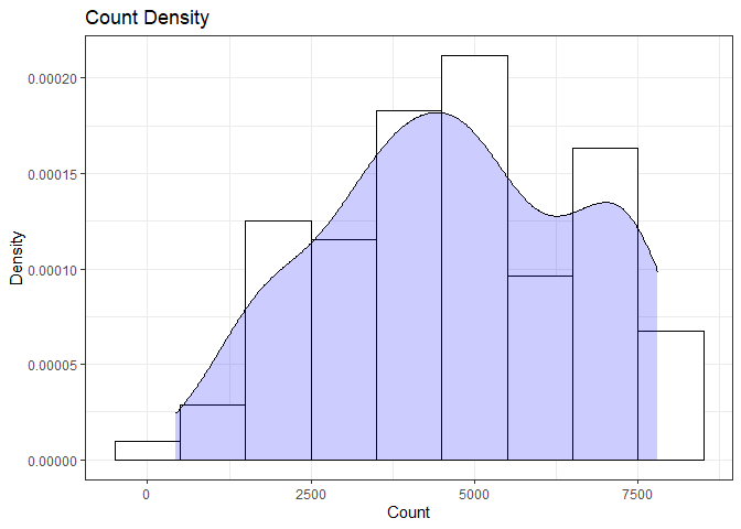
summary(day$cnt)
##    Min. 1st Qu.  Median    Mean 3rd Qu.    Max.
##     431    3271    4721    4667    6286    7804
From the histogram and summary statistics output, it is pretty evident that the count of total rental bikes are in the sub 5000 range. We will investigate if there is a relationship between the response variable and other relevant predictor variables in the next section. Lets look at the other variables individually.
#visualize numeric predictor variables using a histogram
p1 <- ggplot(day) + geom_histogram(aes(x = temp), fill = "red", binwidth = 0.03)
p2 <- ggplot(day) + geom_histogram(aes(x = atemp), fill = "red", binwidth = 0.03)
p3 <- ggplot(day) + geom_histogram(aes(x = hum), fill = "red", binwidth = 0.025)
p4 <- ggplot(day) + geom_histogram(aes(x = windspeed), fill = "red", binwidth = 0.03)
gridExtra::grid.arrange(p1,p2,p3,p4, nrow = 2)
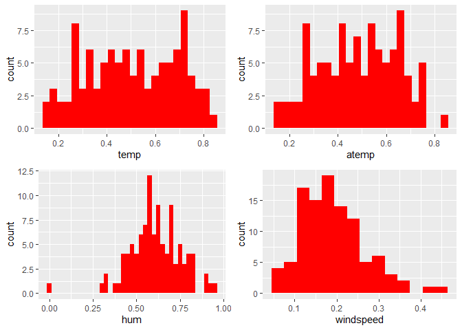
Observations:
* No clear cut pattern in tempand atemp.
-
humappears to be skewed to the left when the dataset is not filtered to a specific weekday. -
windspeedappears to be skewed(right). This variable should be transformed to curb its skewness. -
The distribution of
tempandatemplooks very similar. We should think about taking out one of the variables.
#visualize categorical predictor variables
h1 <- ggplot(day) + geom_bar(aes(x = season),fill = "pink")
h2 <- ggplot(day) + geom_bar(aes(x = yr),fill = "pink")
h3 <- ggplot(day) + geom_bar(aes(x = holiday),fill = "pink")
h4 <- ggplot(day) + geom_bar(aes(x = workingday),fill = "pink")
h5 <- ggplot(day) + geom_bar(aes(x = mnth),fill = "pink")
h6 <- ggplot(day) + geom_bar(aes(x = weathersit),fill = "pink")
gridExtra::grid.arrange(h1,h2,h3,h4,h5,h6, nrow = 3)
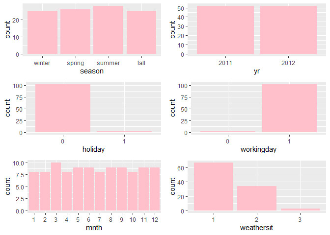
Observations:
* The variation between the four seasons is little to none.
-
About the same number of people rode bikes in 2011 and 2012.
-
Many people rode bikes on days that are not holidays.
-
Most people used the bike-sharing system on days that were neither weekends nor holidays.
-
Most people used the bike sharing system on days with clear weather.
Bi-variate Analysis
In this section, we will explore the predictor variables with respect to the response variable. The objective is to discover hidden relationships between the independent and response variables and use those findings in the model building process.
# First, we will explore the relationship between the target and numerical variables.
p1 <- ggplot(day) +geom_point(aes(x = temp, y = cnt), colour = "violet") + labs(title = "Normalized Temperature vs Total Rental Bikes")
p2 <- ggplot(day) +geom_point(aes(x = atemp, y = cnt), colour = "#FF99CC") +labs(title = "Normalized Feeling Temperature vs Total Rental Bikes")
p3 <- ggplot(day) +geom_point(aes(x = hum, y = cnt), colour = "pink") + labs(title = "Normalized Humidity vs Total rental Bikes")
p4 <- ggplot(day) +geom_point(aes(x = windspeed, y = cnt), colour = "#FF66CC") +labs(title= "Normalized Windspeed vs Total rental Bikes")
gridExtra::grid.arrange(p1, p2, p3, p4, nrow = 2)
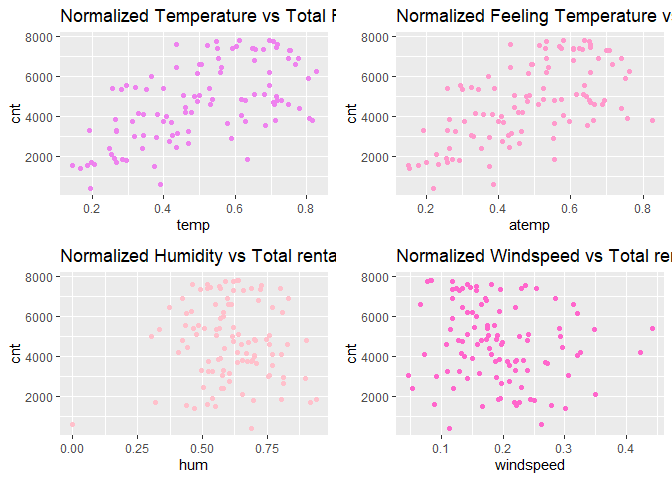
Observations:
* There appears to be a positive linear relationship between cnt ,
temp, and atemp.
- There is also a weak relationship between
cnt,hum, andwindspeed.
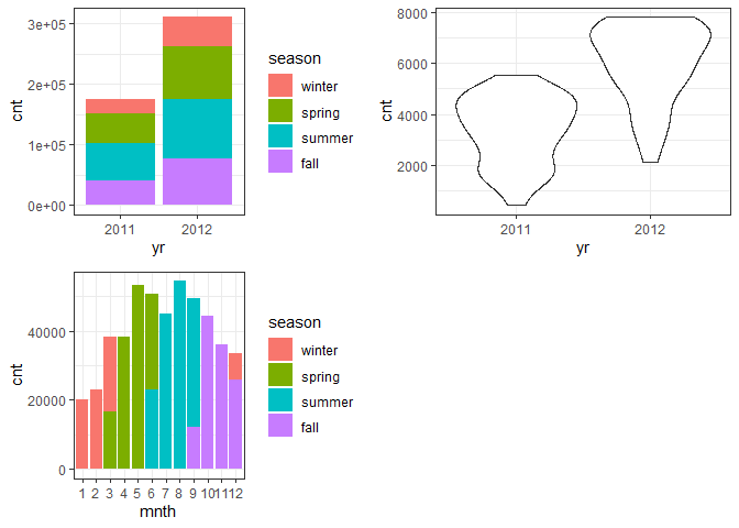
# Now we'll visualize the relationship between the target and categorical variables.
# Instead of using a boxplot, I will use a violin plot which is the blend of both a boxplot and density plot
g1 <- ggplot(day) + geom_col(aes(x = yr, y = cnt, fill = season))+theme_bw()
g2 <- ggplot(day) + geom_violin(aes(x = yr, y = cnt))+theme_bw()
g3 <- ggplot(day) + geom_col(aes(x = mnth, y = cnt, fill = season))+theme_bw()
g4 <- ggplot(day) + geom_col(aes(x = holiday, y = cnt, fill = season)) + theme_bw()
g6 <- ggplot(day) + geom_col(aes(x = workingday, y = cnt, fill = season))
g7 <- ggplot(day) + geom_col(aes(x = weathersit, y = cnt, fill = season))
gridExtra::grid.arrange(g1, g2, g3, nrow = 2)
gridExtra::grid.arrange(g4, g6, g7, nrow = 2)
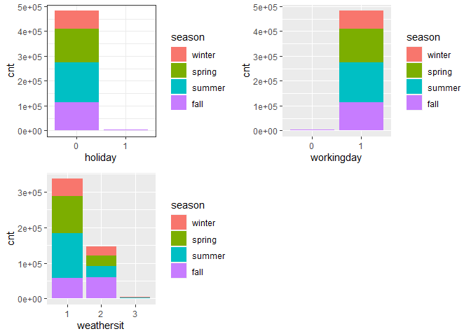 Observations:
* The total bike rental count is higher in 2012 than 2011.
-
During workingday, the bike rental counts quite the highest compared to during no working day for different seasons.
-
During clear,partly cloudy weather, the bike rental count is highest and the second highest is during mist cloudy weather and followed by third highest during light snow and light rain weather.
-
The highest bike rental count was during the summer and lowest in the winter.
Correlation Matrix
Correlation matrix helps us to understand the linear relationship between variables.
day_c <- day[ , c(10:14)]
round(cor(day_c), 2)
##            temp atemp   hum windspeed   cnt
## temp       1.00  1.00  0.15     -0.11  0.60
## atemp      1.00  1.00  0.15     -0.12  0.61
## hum        0.15  0.15  1.00     -0.31  0.00
## windspeed -0.11 -0.12 -0.31      1.00 -0.18
## cnt        0.60  0.61  0.00     -0.18  1.00
From the above matrix, we can see that temp and atemp are highly
correlated. So we only need to include one of these variables in the
model to prevent multicollinearity. We will also transform the humidity
and windspeed variable.
day <- mutate(day, log_hum = log(day$hum+1))
day <- mutate(day, log_ws = log(day$windspeed + 1))

#Remove irrelevant variables
day <- select(day, -weekday,-holiday,-workingday,-dteday,-temp, -instant)
Model Building
First we split the data into train and test sets.
set.seed(23)
dayIndex<- createDataPartition(day$cnt, p = 0.7, list=FALSE)
dayTrain <- day[dayIndex, ]
dayTest <- day[-dayIndex, ]

# Build a tree-based model using loocv;
fitTree <- train(cnt~ ., data = dayTrain, method = "rpart",
              preProcess = c("center", "scale"),
              trControl = trainControl(method = "loocv", number = 10), tuneGrid = data.frame(cp = 0.01:0.10))
## Warning in nominalTrainWorkflow(x = x, y = y, wts = weights, info =
## trainInfo, : There were missing values in resampled performance measures.
# Build a boosted tree model using cv
fitBoost <- train(cnt~., data = dayTrain, method = "gbm",
              preProcess = c("center", "scale"),
              trControl = trainControl(method = "cv", number = 10),
              tuneGrid = expand.grid(n.trees=c(10,20,50,100,500,1000),shrinkage=c(0.01,0.05,0.1,0.5),n.minobsinnode =c(3,5,10),interaction.depth=c(1,5,10)))

# Adding a linear regression model part 2!
FitLinear <- train(cnt~ atemp + mnth*season, data = dayTrain, method = "lm", trControl = trainControl(method = "cv", number = 10))
## Warning in predict.lm(modelFit, newdata): prediction from a rank-deficient
## fit may be misleading

## Warning in predict.lm(modelFit, newdata): prediction from a rank-deficient
## fit may be misleading

## Warning in predict.lm(modelFit, newdata): prediction from a rank-deficient
## fit may be misleading

## Warning in predict.lm(modelFit, newdata): prediction from a rank-deficient
## fit may be misleading

## Warning in predict.lm(modelFit, newdata): prediction from a rank-deficient
## fit may be misleading

## Warning in predict.lm(modelFit, newdata): prediction from a rank-deficient
## fit may be misleading

## Warning in predict.lm(modelFit, newdata): prediction from a rank-deficient
## fit may be misleading

## Warning in predict.lm(modelFit, newdata): prediction from a rank-deficient
## fit may be misleading

## Warning in predict.lm(modelFit, newdata): prediction from a rank-deficient
## fit may be misleading

## Warning in predict.lm(modelFit, newdata): prediction from a rank-deficient
## fit may be misleading
# Display information from the tree fit
fitTree$results
##     cp     RMSE Rsquared      MAE  RMSESD RsquaredSD   MAESD
## 1 0.01 743.4704      NaN 743.4704 549.294         NA 549.294
# Display information from the boost fit
fitBoost$results
##     shrinkage interaction.depth n.minobsinnode n.trees      RMSE
## 1        0.01                 1              3      10 1864.2717
## 7        0.01                 1              5      10 1859.1855
## 13       0.01                 1             10      10 1856.9184
## 55       0.05                 1              3      10 1573.7036
## 61       0.05                 1              5      10 1584.0698
## 67       0.05                 1             10      10 1568.6605
## 109      0.10                 1              3      10 1329.4001
## 115      0.10                 1              5      10 1317.8019
## 121      0.10                 1             10      10 1309.9015
## 163      0.50                 1              3      10  886.9316
## 169      0.50                 1              5      10  866.4506
## 175      0.50                 1             10      10  884.0415
## 19       0.01                 5              3      10 1791.4768
## 25       0.01                 5              5      10 1795.3819
## 31       0.01                 5             10      10 1840.7325
## 73       0.05                 5              3      10 1359.7522
## 79       0.05                 5              5      10 1371.5183
## 85       0.05                 5             10      10 1533.4310
## 127      0.10                 5              3      10 1049.6298
## 133      0.10                 5              5      10 1080.8109
## 139      0.10                 5             10      10 1237.6569
## 181      0.50                 5              3      10 1021.1574
## 187      0.50                 5              5      10 1013.1553
## 193      0.50                 5             10      10  975.4051
## 37       0.01                10              3      10 1784.1118
## 43       0.01                10              5      10 1793.8931
## 49       0.01                10             10      10 1848.2704
## 91       0.05                10              3      10 1342.0240
## 97       0.05                10              5      10 1359.8055
## 103      0.05                10             10      10 1527.7376
## 145      0.10                10              3      10 1036.4113
## 151      0.10                10              5      10 1056.8787
## 157      0.10                10             10      10 1265.3914
## 199      0.50                10              3      10  935.0965
## 205      0.50                10              5      10  908.0440
## 211      0.50                10             10      10  954.5297
## 2        0.01                 1              3      20 1789.8489
## 8        0.01                 1              5      20 1781.4054
## 14       0.01                 1             10      20 1780.8002
## 56       0.05                 1              3      20 1310.0714
## 62       0.05                 1              5      20 1330.9904
## 68       0.05                 1             10      20 1330.8677
## 110      0.10                 1              3      20 1060.8307
## 116      0.10                 1              5      20 1052.1111
## 122      0.10                 1             10      20 1018.6292
## 164      0.50                 1              3      20  873.7788
## 170      0.50                 1              5      20  856.6444
## 176      0.50                 1             10      20  869.4446
## 20       0.01                 5              3      20 1665.1547
## 26       0.01                 5              5      20 1667.8590
## 32       0.01                 5             10      20 1758.6374
## 74       0.05                 5              3      20 1056.4163
## 80       0.05                 5              5      20 1076.5275
## 86       0.05                 5             10      20 1247.8215
## 128      0.10                 5              3      20  865.4141
## 134      0.10                 5              5      20  887.5663
## 140      0.10                 5             10      20  983.5923
## 182      0.50                 5              3      20 1020.9626
## 188      0.50                 5              5      20  984.2517
## 194      0.50                 5             10      20  994.4988
## 38       0.01                10              3      20 1655.9240
## 44       0.01                10              5      20 1669.3564
## 50       0.01                10             10      20 1758.2268
## 92       0.05                10              3      20 1047.0679
## 98       0.05                10              5      20 1072.0337
## 104      0.05                10             10      20 1266.8659
## 146      0.10                10              3      20  866.8169
## 152      0.10                10              5      20  860.2319
## 158      0.10                10             10      20  974.3931
## 200      0.50                10              3      20  955.0612
## 206      0.50                10              5      20  944.7488
## 212      0.50                10             10      20  978.5716
## 3        0.01                 1              3      50 1588.5217
## 9        0.01                 1              5      50 1582.4048
## 15       0.01                 1             10      50 1579.1655
## 57       0.05                 1              3      50  983.3248
## 63       0.05                 1              5      50  969.4680
## 69       0.05                 1             10      50  958.4021
## 111      0.10                 1              3      50  870.0316
## 117      0.10                 1              5      50  856.0272
## 123      0.10                 1             10      50  867.8476
## 165      0.50                 1              3      50  832.7280
## 171      0.50                 1              5      50  882.3729
## 177      0.50                 1             10      50  865.2674
## 21       0.01                 5              3      50 1365.2866
## 27       0.01                 5              5      50 1370.5749
## 33       0.01                 5             10      50 1534.2965
## 75       0.05                 5              3      50  848.9628
## 81       0.05                 5              5      50  837.0501
## 87       0.05                 5             10      50  927.7656
## 129      0.10                 5              3      50  844.8007
## 135      0.10                 5              5      50  853.2856
## 141      0.10                 5             10      50  908.6849
## 183      0.50                 5              3      50 1021.2704
## 189      0.50                 5              5      50  999.6380
## 195      0.50                 5             10      50  993.6887
## 39       0.01                10              3      50 1345.0391
## 45       0.01                10              5      50 1369.2928
## 51       0.01                10             10      50 1523.2433
## 93       0.05                10              3      50  825.7473
##      Rsquared       MAE   RMSESD RsquaredSD    MAESD
## 1   0.6850362 1557.0873 259.7919 0.23821425 233.9136
## 7   0.6770674 1554.3057 255.7712 0.22778344 232.8825
## 13  0.7026600 1552.7993 257.1232 0.22054134 234.7776
## 55  0.8044346 1320.5327 248.1262 0.12326276 207.6607
## 61  0.7522646 1331.0857 234.7315 0.15387063 193.7389
## 67  0.7918185 1313.0928 255.1850 0.16001968 208.6948
## 109 0.8008040 1118.0599 224.7328 0.12429592 171.0893
## 115 0.8059472 1108.8350 233.9083 0.09185174 179.8859
## 121 0.7941981 1114.6447 252.4193 0.13970426 182.0970
## 163 0.8045052  733.5306 303.7877 0.10962122 258.4939
## 169 0.8362973  700.5930 283.1843 0.09822091 257.1315
## 175 0.8442761  703.2544 271.0804 0.09697533 215.4204
## 19  0.8469675 1494.5855 257.7303 0.09256857 229.5802
## 25  0.8182094 1498.2125 260.2189 0.09783715 230.9728
## 31  0.7274171 1536.1717 256.3627 0.18035006 236.7624
## 73  0.8477475 1138.3264 280.3673 0.07446189 210.4906
## 79  0.8424323 1150.8571 256.2669 0.09290149 201.6582
## 85  0.7856187 1289.9711 240.6970 0.15676727 193.0515
## 127 0.8395794  877.4171 343.3042 0.09671781 280.1285
## 133 0.8121061  923.3848 265.6403 0.10845129 217.7490
## 139 0.7989906 1045.0780 254.4013 0.12026414 199.7915
## 181 0.8093978  840.9716 421.6900 0.15402233 357.4629
## 187 0.7770235  839.3477 313.8983 0.14422086 224.1257
## 193 0.8096482  794.2282 260.9296 0.12283835 202.0078
## 37  0.8298605 1485.0968 259.8199 0.09663022 232.7854
## 43  0.8198029 1496.2719 260.0776 0.10313373 233.2397
## 49  0.6933679 1545.3698 257.6950 0.26169328 236.0194
## 91  0.8561996 1132.0101 277.7758 0.07244660 221.0985
## 97  0.8374431 1141.1931 262.3506 0.08619282 202.0808
## 103 0.8045970 1277.3548 248.0613 0.13161180 188.6034
## 145 0.8474893  880.6428 328.4162 0.09704466 268.9566
## 151 0.8505588  903.8331 277.3976 0.08416008 232.8118
## 157 0.8125081 1068.1620 270.5805 0.09900329 196.7793
## 199 0.8200527  762.3805 332.1242 0.16745529 247.7656
## 205 0.8174984  730.4146 314.0029 0.11538987 234.4330
## 211 0.8249891  741.7643 248.7130 0.10531057 223.6690
## 2   0.7401346 1496.8207 258.2144 0.21819672 229.4823
## 8   0.7556816 1488.9669 251.9581 0.16981264 225.4548
## 14  0.7627547 1486.8176 257.6105 0.17070186 229.2745
## 56  0.8374055 1108.4165 249.4047 0.09449474 191.3468
## 62  0.8023965 1128.5991 260.0513 0.12303861 201.5763
## 68  0.8026870 1121.3550 238.3621 0.13157340 174.5720
## 110 0.8149086  904.1516 249.3768 0.11309390 217.1498
## 116 0.8139718  875.4168 256.3713 0.11005717 215.3771
## 122 0.8306009  867.7938 236.6323 0.11460532 179.5676
## 164 0.8170933  724.0526 302.0556 0.09818684 216.3726
## 170 0.8494752  711.1252 267.2554 0.09194352 224.5239
## 176 0.8465899  705.5593 190.4975 0.08216075 128.7989
## 20  0.8484688 1389.8096 260.9982 0.09006339 223.8419
## 26  0.8408916 1393.4909 262.8389 0.08570910 223.5202
## 32  0.7740827 1470.4317 255.1284 0.12464707 221.8104
## 74  0.8534873  895.9486 299.2160 0.07743279 226.1295
## 80  0.8419777  904.8748 279.2614 0.07870377 221.1419
## 86  0.8283536 1062.7162 215.4862 0.10107949 151.8962
## 128 0.8587335  701.7134 326.1752 0.06749806 247.4103
## 134 0.8334847  746.8247 290.1476 0.09025514 238.2728
## 140 0.8262476  831.2629 236.7217 0.08325589 198.2533
## 182 0.8011528  803.8320 396.4684 0.14378856 302.6131
## 188 0.7963460  797.7705 276.1068 0.12797995 216.6766
## 194 0.7877547  809.9706 220.7838 0.13745490 192.4304
## 38  0.8463839 1381.7782 265.0581 0.07910371 222.5957
## 44  0.8238623 1393.9399 267.9728 0.10099436 226.2909
## 50  0.7658254 1474.4770 257.2698 0.16984437 220.5050
## 92  0.8626562  903.1955 312.1963 0.06961327 237.4153
## 98  0.8386615  907.3394 270.3442 0.08328089 210.0014
## 104 0.8001023 1068.9197 251.6672 0.14834315 187.6868
## 146 0.8441951  709.9149 315.9491 0.10093242 233.5761
## 152 0.8522629  724.0069 264.1347 0.08898044 215.6574
## 158 0.8323857  838.5853 258.6550 0.08880176 209.3515
## 200 0.8070910  771.7706 359.5311 0.18678152 265.3135
## 206 0.7944286  761.0974 310.8926 0.12678095 257.5970
## 212 0.8212862  780.0751 221.1031 0.07949321 179.8327
## 3   0.8042614 1326.7942 257.7728 0.12095817 207.4785
## 9   0.7961653 1324.5721 249.0079 0.12426299 199.0289
## 15  0.8066676 1318.7621 252.7541 0.12485901 203.1001
## 57  0.8305954  827.4170 243.1057 0.08917993 187.7344
## 63  0.8272960  825.0108 271.7480 0.10459350 224.6430
## 69  0.8333180  817.6068 232.8389 0.09874151 192.6296
## 111 0.8321799  714.7083 295.5219 0.09482054 244.2267
## 117 0.8417653  701.1455 299.3435 0.08561637 239.1377
## 123 0.8479585  710.1546 234.9020 0.08035307 191.2346
## 165 0.8345589  679.1408 271.3281 0.09849049 223.0987
## 171 0.8500628  735.5200 238.5992 0.09286884 201.5154
## 177 0.8488439  717.7710 195.8752 0.07845761 178.2870
## 21  0.8520707 1140.1573 284.7544 0.08226815 213.7216
## 27  0.8407730 1150.7215 263.8294 0.08539107 203.7814
## 33  0.8154026 1285.6022 252.7921 0.10518535 194.5379
## 75  0.8482413  687.9903 318.5668 0.08942258 246.2875
## 81  0.8544699  684.7919 292.6316 0.07749202 242.9154
## 87  0.8371546  790.6991 227.4526 0.08434788 186.4946
## 129 0.8502375  678.2367 297.5333 0.08863218 214.2636
## 135 0.8435135  697.8207 267.9258 0.09055415 204.3096
## 141 0.8289061  749.4758 214.2314 0.08144627 189.1945
## 183 0.8016083  800.4457 390.5882 0.13397298 289.3027
## 189 0.7810432  835.2504 255.7182 0.12764437 186.9562
## 195 0.7660926  810.6875 280.5712 0.15075305 250.8209
## 39  0.8543123 1125.4805 287.3554 0.07345144 217.8715
## 45  0.8325284 1150.5047 263.9487 0.08375723 201.9086
## 51  0.8246177 1275.5384 253.6353 0.11019558 196.5753
## 93  0.8692448  671.7572 295.6295 0.06598719 234.7997
##  [ reached 'max' / getOption("max.print") -- omitted 116 rows ]
# Display information from the linear model fit
FitLinear$results
##   intercept     RMSE  Rsquared      MAE   RMSESD RsquaredSD    MAESD
## 1      TRUE 1829.995 0.2404472 1552.775 401.3863  0.1471392 430.8601
Now, we make predictions on the test data sets using the best model fits. Then we compare RMSE to determine the best model.
predTree <- predict(fitTree, newdata = select(dayTest, -cnt))
postResample(predTree, dayTest$cnt)
##         RMSE     Rsquared          MAE
## 1267.2719351    0.6313671 1017.6188560
boostPred <- predict(fitBoost, newdata = select(dayTest, -cnt))
postResample(boostPred, dayTest$cnt)
##        RMSE    Rsquared         MAE
## 854.1404587   0.7908244 633.0513930
linearPred <- predict(FitLinear, newdata = select(dayTest, -cnt))
## Warning in predict.lm(modelFit, newdata): prediction from a rank-deficient
## fit may be misleading
postResample(linearPred, dayTest$cnt)
##         RMSE     Rsquared          MAE
## 1462.1790208    0.3857482 1252.8251840
When we compare the two models, the boosted tree model has lower RMSE values when applied on the test dataset. Hence, the boosted tree model is our final model and best model for interpreting the bike rental count on a daily basis.