Project 2
Ifeoma Ojialor 10/16/2020
Introduction
In this project, we will use a bike-sharing dataset to create machine
learning models. Before moving forward, I will briefly explain the
bike-sharing system and how it works. A bike-sharing system is a service
in which users can rent/use bicycles on a short term basis for a fee.
The goal of these programs is to provide affordable access to bicycles
for short distance trips as opposed to walking or taking public
transportation. Imagine how many people use these systems on a given
day, the numbers can vary greatly based on some elements. The goal of
this project is to build a predictive model to find out the number of
people that use these bikes in a given time period using available
information about that time/day. This in turn, can help businesses that
oversee this systems to manage them in a cost efficient manner.
We will be using the bike-sharing dataset from the UCL Machine Learning
Repository. We will use the regression and boosted tree method to model
the response variable cnt.
Exploratory Data Analysis
First we will read in the data using a relative path.
#read in data and filter to desired weekday
day1 <- read.csv("Bike-Sharing-Dataset/day.csv")
head(day1,5)
##   instant     dteday season yr mnth holiday weekday workingday weathersit
## 1       1 2011-01-01      1  0    1       0       6          0          2
## 2       2 2011-01-02      1  0    1       0       0          0          2
## 3       3 2011-01-03      1  0    1       0       1          1          1
## 4       4 2011-01-04      1  0    1       0       2          1          1
## 5       5 2011-01-05      1  0    1       0       3          1          1
##       temp    atemp      hum windspeed casual registered  cnt
## 1 0.344167 0.363625 0.805833  0.160446    331        654  985
## 2 0.363478 0.353739 0.696087  0.248539    131        670  801
## 3 0.196364 0.189405 0.437273  0.248309    120       1229 1349
## 4 0.200000 0.212122 0.590435  0.160296    108       1454 1562
## 5 0.226957 0.229270 0.436957  0.186900     82       1518 1600
Next, we will remove the casual and registered variables since the
cnt variable is a combination of both.
day1 <- select(day1, -casual, -registered)
day1$weekday <- as.factor(day1$weekday)
levels(day1$weekday) <- c("Sunday", "Monday", "Tuesday", "Wednesday", "Thursday", "Friday", "Saturday")
day <- filter(day1, weekday == params$days)

#Check for missing values
miss <- data.frame(apply(day,2,function(x){sum(is.na(x))}))
names(miss)[1] <- "missing"
miss
##            missing
## instant          0
## dteday           0
## season           0
## yr               0
## mnth             0
## holiday          0
## weekday          0
## workingday       0
## weathersit       0
## temp             0
## atemp            0
## hum              0
## windspeed        0
## cnt              0
There are no missing values in the dataset, so we can continue with our analysis.
#Change the variables into their appropriate format.
day$season <- as.factor(day$season)
day$weathersit <- as.factor(day$weathersit)
day$holiday <- as.factor(day$holiday)
day$workingday <- as.factor(day$workingday)
day$yr <- as.factor(day$yr)
day$mnth <- as.factor(day$mnth)

levels(day$season) <- c("winter", "spring", "summer", "fall")
levels(day$yr) <- c("2011", "2012")
str(day)
## 'data.frame':    105 obs. of  14 variables:
##  $ instant   : int  3 10 17 24 31 38 45 52 59 66 ...
##  $ dteday    : chr  "2011-01-03" "2011-01-10" "2011-01-17" "2011-01-24" ...
##  $ season    : Factor w/ 4 levels "winter","spring",..: 1 1 1 1 1 1 1 1 1 1 ...
##  $ yr        : Factor w/ 2 levels "2011","2012": 1 1 1 1 1 1 1 1 1 1 ...
##  $ mnth      : Factor w/ 12 levels "1","2","3","4",..: 1 1 1 1 1 2 2 2 2 3 ...
##  $ holiday   : Factor w/ 2 levels "0","1": 1 1 2 1 1 1 1 2 1 1 ...
##  $ weekday   : Factor w/ 7 levels "Sunday","Monday",..: 2 2 2 2 2 2 2 2 2 2 ...
##  $ workingday: Factor w/ 2 levels "0","1": 2 2 1 2 2 2 2 1 2 2 ...
##  $ weathersit: Factor w/ 3 levels "1","2","3": 1 1 2 1 2 1 1 2 2 1 ...
##  $ temp      : num  0.1964 0.1508 0.1758 0.0974 0.1808 ...
##  $ atemp     : num  0.189 0.151 0.177 0.118 0.186 ...
##  $ hum       : num  0.437 0.483 0.537 0.492 0.604 ...
##  $ windspeed : num  0.248 0.223 0.194 0.158 0.187 ...
##  $ cnt       : int  1349 1321 1000 1416 1501 1712 1913 1107 1446 1872 ...
Univariate Analysis
The cnt is the response variable, so we’ll use a histogram to get a
visual understanding of the variable.
ggplot(day, aes(x = cnt)) + theme_bw() + geom_histogram(aes(y =..density..), color = "black", fill = "white", binwidth = 1000) + geom_density(alpha = 0.2, fill = "blue") + labs(title = "Count Density", x = "Count", y = "Density")
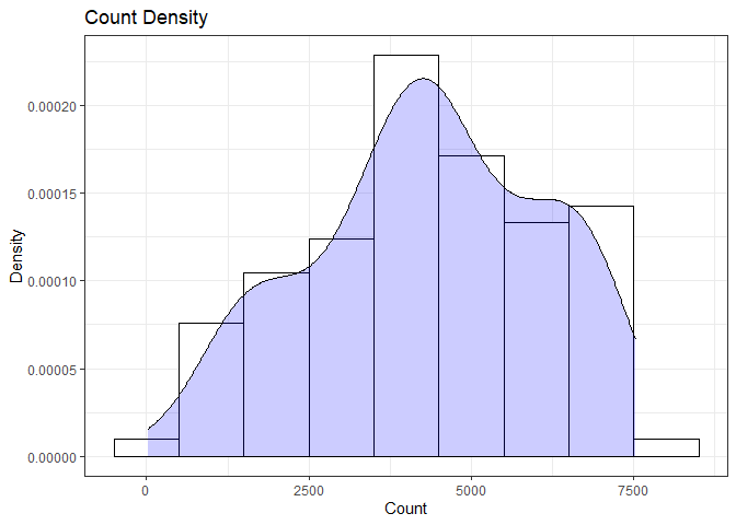
summary(day$cnt)
##    Min. 1st Qu.  Median    Mean 3rd Qu.    Max.
##      22    3310    4359    4338    5875    7525
From the histogram and summary statistics output, it is pretty evident that the count of total rental bikes are in the sub 5000 range. We will investigate if there is a relationship between the response variable and other relevant predictor variables in the next section. Lets look at the other variables individually.
#visualize numeric predictor variables using a histogram
p1 <- ggplot(day) + geom_histogram(aes(x = temp), fill = "red", binwidth = 0.03)
p2 <- ggplot(day) + geom_histogram(aes(x = atemp), fill = "red", binwidth = 0.03)
p3 <- ggplot(day) + geom_histogram(aes(x = hum), fill = "red", binwidth = 0.025)
p4 <- ggplot(day) + geom_histogram(aes(x = windspeed), fill = "red", binwidth = 0.03)
gridExtra::grid.arrange(p1,p2,p3,p4, nrow = 2)
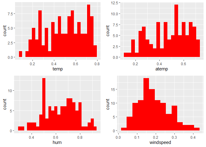
Observations:
* No clear cut pattern in tempand atemp.
-
humappears to be skewed to the left when the dataset is not filtered to a specific weekday. -
windspeedappears to be skewed(right). This variable should be transformed to curb its skewness. -
The distribution of
tempandatemplooks very similar. We should think about taking out one of the variables.
#visualize categorical predictor variables
h1 <- ggplot(day) + geom_bar(aes(x = season),fill = "pink")
h2 <- ggplot(day) + geom_bar(aes(x = yr),fill = "pink")
h3 <- ggplot(day) + geom_bar(aes(x = holiday),fill = "pink")
h4 <- ggplot(day) + geom_bar(aes(x = workingday),fill = "pink")
h5 <- ggplot(day) + geom_bar(aes(x = mnth),fill = "pink")
h6 <- ggplot(day) + geom_bar(aes(x = weathersit),fill = "pink")
gridExtra::grid.arrange(h1,h2,h3,h4,h5,h6, nrow = 3)
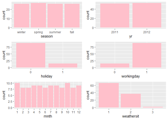
Observations:
* The variation between the four seasons is little to none.
-
About the same number of people rode bikes in 2011 and 2012.
-
Many people rode bikes on days that are not holidays.
-
Most people used the bike-sharing system on days that were neither weekends nor holidays.
-
Most people used the bike sharing system on days with clear weather.
Bi-variate Analysis
In this section, we will explore the predictor variables with respect to the response variable. The objective is to discover hidden relationships between the independent and response variables and use those findings in the model building process.
# First, we will explore the relationship between the target and numerical variables.
p1 <- ggplot(day) +geom_point(aes(x = temp, y = cnt), colour = "violet") + labs(title = "Normalized Temperature vs Total Rental Bikes")
p2 <- ggplot(day) +geom_point(aes(x = atemp, y = cnt), colour = "#FF99CC") +labs(title = "Normalized Feeling Temperature vs Total Rental Bikes")
p3 <- ggplot(day) +geom_point(aes(x = hum, y = cnt), colour = "pink") + labs(title = "Normalized Humidity vs Total rental Bikes")
p4 <- ggplot(day) +geom_point(aes(x = windspeed, y = cnt), colour = "#FF66CC") +labs(title= "Normalized Windspeed vs Total rental Bikes")
gridExtra::grid.arrange(p1, p2, p3, p4, nrow = 2)
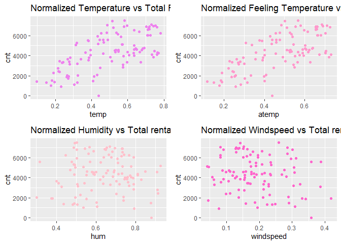
Observations:
* There appears to be a positive linear relationship between cnt ,
temp, and atemp.
- There is also a weak relationship between
cnt,hum, andwindspeed.
# Now we'll visualize the relationship between the target and categorical variables.
# Instead of using a boxplot, I will use a violin plot which is the blend of both a boxplot and density plot
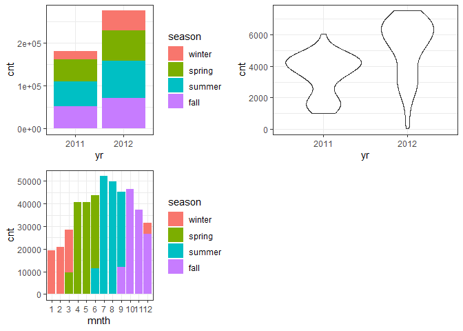
g1 <- ggplot(day) + geom_col(aes(x = yr, y = cnt, fill = season))+theme_bw()
g2 <- ggplot(day) + geom_violin(aes(x = yr, y = cnt))+theme_bw()
g3 <- ggplot(day) + geom_col(aes(x = mnth, y = cnt, fill = season))+theme_bw()
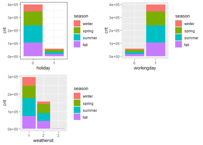
g4 <- ggplot(day) + geom_col(aes(x = holiday, y = cnt, fill = season)) + theme_bw()
g6 <- ggplot(day) + geom_col(aes(x = workingday, y = cnt, fill = season))
g7 <- ggplot(day) + geom_col(aes(x = weathersit, y = cnt, fill = season))
gridExtra::grid.arrange(g1, g2, g3, nrow = 2)
gridExtra::grid.arrange(g4, g6, g7, nrow = 2)
 Observations:
* The total bike rental count is higher in 2012 than 2011.
-
During workingday, the bike rental counts quite the highest compared to during no working day for different seasons.
-
During clear,partly cloudy weather, the bike rental count is highest and the second highest is during mist cloudy weather and followed by third highest during light snow and light rain weather.
-
The highest bike rental count was during the summer and lowest in the winter.
Correlation Matrix
Correlation matrix helps us to understand the linear relationship between variables.
day_c <- day[ , c(10:14)]
round(cor(day_c), 2)
##            temp atemp   hum windspeed   cnt
## temp       1.00  1.00  0.19     -0.03  0.65
## atemp      1.00  1.00  0.22     -0.06  0.67
## hum        0.19  0.22  1.00     -0.42  0.00
## windspeed -0.03 -0.06 -0.42      1.00 -0.17
## cnt        0.65  0.67  0.00     -0.17  1.00
From the above matrix, we can see that temp and atemp are highly
correlated. So we only need to include one of these variables in the
model to prevent multicollinearity. We will also transform the humidity
and windspeed variable.
day <- mutate(day, log_hum = log(day$hum+1))
day <- mutate(day, log_ws = log(day$windspeed + 1))

#Remove irrelevant variables
day <- select(day, -weekday,-holiday,-workingday,-dteday,-temp, -instant)
Model Building
First we split the data into train and test sets.
set.seed(23)
dayIndex<- createDataPartition(day$cnt, p = 0.7, list=FALSE)
dayTrain <- day[dayIndex, ]
dayTest <- day[-dayIndex, ]

# Build a tree-based model using loocv;
fitTree <- train(cnt~ ., data = dayTrain, method = "rpart",
              preProcess = c("center", "scale"),
              trControl = trainControl(method = "loocv", number = 10), tuneGrid = data.frame(cp = 0.01:0.10))
## Warning in preProcess.default(thresh = 0.95, k = 5, freqCut = 19,
## uniqueCut = 10, : These variables have zero variances: weathersit3

## Warning in nominalTrainWorkflow(x = x, y = y, wts = weights, info =
## trainInfo, : There were missing values in resampled performance measures.
# Build a boosted tree model using cv
fitBoost <- train(cnt~., data = dayTrain, method = "gbm",
              preProcess = c("center", "scale"),
              trControl = trainControl(method = "cv", number = 10),
              tuneGrid = expand.grid(n.trees=c(10,20,50,100,500,1000),shrinkage=c(0.01,0.05,0.1,0.5),n.minobsinnode =c(3,5,10),interaction.depth=c(1,5,10)))
## Warning in preProcess.default(thresh = 0.95, k = 5, freqCut = 19,
## uniqueCut = 10, : These variables have zero variances: weathersit3

## Warning in (function (x, y, offset = NULL, misc = NULL, distribution =
## "bernoulli", : variable 17: weathersit3 has no variation.

## Warning in preProcess.default(thresh = 0.95, k = 5, freqCut = 19,
## uniqueCut = 10, : These variables have zero variances: weathersit3

## Warning in (function (x, y, offset = NULL, misc = NULL, distribution =
## "bernoulli", : variable 17: weathersit3 has no variation.

## Warning in preProcess.default(thresh = 0.95, k = 5, freqCut = 19,
## uniqueCut = 10, : These variables have zero variances: weathersit3

## Warning in (function (x, y, offset = NULL, misc = NULL, distribution =
## "bernoulli", : variable 17: weathersit3 has no variation.

## Warning in preProcess.default(thresh = 0.95, k = 5, freqCut = 19,
## uniqueCut = 10, : These variables have zero variances: weathersit3

## Warning in (function (x, y, offset = NULL, misc = NULL, distribution =
## "bernoulli", : variable 17: weathersit3 has no variation.

## Warning in preProcess.default(thresh = 0.95, k = 5, freqCut = 19,
## uniqueCut = 10, : These variables have zero variances: weathersit3

## Warning in (function (x, y, offset = NULL, misc = NULL, distribution =
## "bernoulli", : variable 17: weathersit3 has no variation.

## Warning in preProcess.default(thresh = 0.95, k = 5, freqCut = 19,
## uniqueCut = 10, : These variables have zero variances: weathersit3

## Warning in (function (x, y, offset = NULL, misc = NULL, distribution =
## "bernoulli", : variable 17: weathersit3 has no variation.

## Warning in preProcess.default(thresh = 0.95, k = 5, freqCut = 19,
## uniqueCut = 10, : These variables have zero variances: weathersit3

## Warning in (function (x, y, offset = NULL, misc = NULL, distribution =
## "bernoulli", : variable 17: weathersit3 has no variation.

## Warning in preProcess.default(thresh = 0.95, k = 5, freqCut = 19,
## uniqueCut = 10, : These variables have zero variances: weathersit3

## Warning in (function (x, y, offset = NULL, misc = NULL, distribution =
## "bernoulli", : variable 17: weathersit3 has no variation.

## Warning in preProcess.default(thresh = 0.95, k = 5, freqCut = 19,
## uniqueCut = 10, : These variables have zero variances: weathersit3

## Warning in (function (x, y, offset = NULL, misc = NULL, distribution =
## "bernoulli", : variable 17: weathersit3 has no variation.

## Warning in preProcess.default(thresh = 0.95, k = 5, freqCut = 19,
## uniqueCut = 10, : These variables have zero variances: weathersit3

## Warning in (function (x, y, offset = NULL, misc = NULL, distribution =
## "bernoulli", : variable 17: weathersit3 has no variation.

## Warning in preProcess.default(thresh = 0.95, k = 5, freqCut = 19,
## uniqueCut = 10, : These variables have zero variances: weathersit3

## Warning in (function (x, y, offset = NULL, misc = NULL, distribution =
## "bernoulli", : variable 17: weathersit3 has no variation.

## Warning in preProcess.default(thresh = 0.95, k = 5, freqCut = 19,
## uniqueCut = 10, : These variables have zero variances: weathersit3

## Warning in (function (x, y, offset = NULL, misc = NULL, distribution =
## "bernoulli", : variable 17: weathersit3 has no variation.

## Warning in preProcess.default(thresh = 0.95, k = 5, freqCut = 19,
## uniqueCut = 10, : These variables have zero variances: weathersit3

## Warning in (function (x, y, offset = NULL, misc = NULL, distribution =
## "bernoulli", : variable 17: weathersit3 has no variation.

## Warning in preProcess.default(thresh = 0.95, k = 5, freqCut = 19,
## uniqueCut = 10, : These variables have zero variances: weathersit3

## Warning in (function (x, y, offset = NULL, misc = NULL, distribution =
## "bernoulli", : variable 17: weathersit3 has no variation.

## Warning in preProcess.default(thresh = 0.95, k = 5, freqCut = 19,
## uniqueCut = 10, : These variables have zero variances: weathersit3

## Warning in (function (x, y, offset = NULL, misc = NULL, distribution =
## "bernoulli", : variable 17: weathersit3 has no variation.

## Warning in preProcess.default(thresh = 0.95, k = 5, freqCut = 19,
## uniqueCut = 10, : These variables have zero variances: weathersit3

## Warning in (function (x, y, offset = NULL, misc = NULL, distribution =
## "bernoulli", : variable 17: weathersit3 has no variation.

## Warning in preProcess.default(thresh = 0.95, k = 5, freqCut = 19,
## uniqueCut = 10, : These variables have zero variances: weathersit3

## Warning in (function (x, y, offset = NULL, misc = NULL, distribution =
## "bernoulli", : variable 17: weathersit3 has no variation.

## Warning in preProcess.default(thresh = 0.95, k = 5, freqCut = 19,
## uniqueCut = 10, : These variables have zero variances: weathersit3

## Warning in (function (x, y, offset = NULL, misc = NULL, distribution =
## "bernoulli", : variable 17: weathersit3 has no variation.

## Warning in preProcess.default(thresh = 0.95, k = 5, freqCut = 19,
## uniqueCut = 10, : These variables have zero variances: weathersit3

## Warning in (function (x, y, offset = NULL, misc = NULL, distribution =
## "bernoulli", : variable 17: weathersit3 has no variation.

## Warning in preProcess.default(thresh = 0.95, k = 5, freqCut = 19,
## uniqueCut = 10, : These variables have zero variances: weathersit3

## Warning in (function (x, y, offset = NULL, misc = NULL, distribution =
## "bernoulli", : variable 17: weathersit3 has no variation.

## Warning in preProcess.default(thresh = 0.95, k = 5, freqCut = 19,
## uniqueCut = 10, : These variables have zero variances: weathersit3

## Warning in (function (x, y, offset = NULL, misc = NULL, distribution =
## "bernoulli", : variable 17: weathersit3 has no variation.

## Warning in preProcess.default(thresh = 0.95, k = 5, freqCut = 19,
## uniqueCut = 10, : These variables have zero variances: weathersit3

## Warning in (function (x, y, offset = NULL, misc = NULL, distribution =
## "bernoulli", : variable 17: weathersit3 has no variation.

## Warning in preProcess.default(thresh = 0.95, k = 5, freqCut = 19,
## uniqueCut = 10, : These variables have zero variances: weathersit3

## Warning in (function (x, y, offset = NULL, misc = NULL, distribution =
## "bernoulli", : variable 17: weathersit3 has no variation.

## Warning in preProcess.default(thresh = 0.95, k = 5, freqCut = 19,
## uniqueCut = 10, : These variables have zero variances: weathersit3

## Warning in (function (x, y, offset = NULL, misc = NULL, distribution =
## "bernoulli", : variable 17: weathersit3 has no variation.

## Warning in preProcess.default(thresh = 0.95, k = 5, freqCut = 19,
## uniqueCut = 10, : These variables have zero variances: weathersit3

## Warning in (function (x, y, offset = NULL, misc = NULL, distribution =
## "bernoulli", : variable 17: weathersit3 has no variation.

## Warning in preProcess.default(thresh = 0.95, k = 5, freqCut = 19,
## uniqueCut = 10, : These variables have zero variances: weathersit3

## Warning in (function (x, y, offset = NULL, misc = NULL, distribution =
## "bernoulli", : variable 17: weathersit3 has no variation.

## Warning in preProcess.default(thresh = 0.95, k = 5, freqCut = 19,
## uniqueCut = 10, : These variables have zero variances: weathersit3

## Warning in (function (x, y, offset = NULL, misc = NULL, distribution =
## "bernoulli", : variable 17: weathersit3 has no variation.

## Warning in preProcess.default(thresh = 0.95, k = 5, freqCut = 19,
## uniqueCut = 10, : These variables have zero variances: weathersit3

## Warning in (function (x, y, offset = NULL, misc = NULL, distribution =
## "bernoulli", : variable 17: weathersit3 has no variation.

## Warning in preProcess.default(thresh = 0.95, k = 5, freqCut = 19,
## uniqueCut = 10, : These variables have zero variances: weathersit3

## Warning in (function (x, y, offset = NULL, misc = NULL, distribution =
## "bernoulli", : variable 17: weathersit3 has no variation.

## Warning in preProcess.default(thresh = 0.95, k = 5, freqCut = 19,
## uniqueCut = 10, : These variables have zero variances: weathersit3

## Warning in (function (x, y, offset = NULL, misc = NULL, distribution =
## "bernoulli", : variable 17: weathersit3 has no variation.

## Warning in preProcess.default(thresh = 0.95, k = 5, freqCut = 19,
## uniqueCut = 10, : These variables have zero variances: weathersit3

## Warning in (function (x, y, offset = NULL, misc = NULL, distribution =
## "bernoulli", : variable 17: weathersit3 has no variation.

## Warning in preProcess.default(thresh = 0.95, k = 5, freqCut = 19,
## uniqueCut = 10, : These variables have zero variances: weathersit3

## Warning in (function (x, y, offset = NULL, misc = NULL, distribution =
## "bernoulli", : variable 17: weathersit3 has no variation.

## Warning in preProcess.default(thresh = 0.95, k = 5, freqCut = 19,
## uniqueCut = 10, : These variables have zero variances: weathersit3

## Warning in (function (x, y, offset = NULL, misc = NULL, distribution =
## "bernoulli", : variable 17: weathersit3 has no variation.

## Warning in preProcess.default(thresh = 0.95, k = 5, freqCut = 19,
## uniqueCut = 10, : These variables have zero variances: weathersit3

## Warning in (function (x, y, offset = NULL, misc = NULL, distribution =
## "bernoulli", : variable 17: weathersit3 has no variation.

## Warning in preProcess.default(thresh = 0.95, k = 5, freqCut = 19,
## uniqueCut = 10, : These variables have zero variances: weathersit3

## Warning in (function (x, y, offset = NULL, misc = NULL, distribution =
## "bernoulli", : variable 17: weathersit3 has no variation.

## Warning in preProcess.default(thresh = 0.95, k = 5, freqCut = 19,
## uniqueCut = 10, : These variables have zero variances: weathersit3

## Warning in (function (x, y, offset = NULL, misc = NULL, distribution =
## "bernoulli", : variable 17: weathersit3 has no variation.
# Adding a linear regression model part 2!
FitLinear <- train(cnt~ atemp + mnth*season, data = dayTrain, method = "lm", trControl = trainControl(method = "cv", number = 10))
## Warning in predict.lm(modelFit, newdata): prediction from a rank-deficient
## fit may be misleading

## Warning in predict.lm(modelFit, newdata): prediction from a rank-deficient
## fit may be misleading

## Warning in predict.lm(modelFit, newdata): prediction from a rank-deficient
## fit may be misleading

## Warning in predict.lm(modelFit, newdata): prediction from a rank-deficient
## fit may be misleading

## Warning in predict.lm(modelFit, newdata): prediction from a rank-deficient
## fit may be misleading

## Warning in predict.lm(modelFit, newdata): prediction from a rank-deficient
## fit may be misleading

## Warning in predict.lm(modelFit, newdata): prediction from a rank-deficient
## fit may be misleading

## Warning in predict.lm(modelFit, newdata): prediction from a rank-deficient
## fit may be misleading

## Warning in predict.lm(modelFit, newdata): prediction from a rank-deficient
## fit may be misleading

## Warning in predict.lm(modelFit, newdata): prediction from a rank-deficient
## fit may be misleading
# Display information from the tree fit
fitTree$results
##     cp     RMSE Rsquared      MAE   RMSESD RsquaredSD    MAESD
## 1 0.01 869.1544      NaN 869.1544 937.8054         NA 937.8054
# Display information from the boost fit
fitBoost$results
##     shrinkage interaction.depth n.minobsinnode n.trees      RMSE
## 1        0.01                 1              3      10 1736.6757
## 7        0.01                 1              5      10 1737.6601
## 13       0.01                 1             10      10 1735.6652
## 55       0.05                 1              3      10 1556.1784
## 61       0.05                 1              5      10 1550.5657
## 67       0.05                 1             10      10 1543.7300
## 109      0.10                 1              3      10 1382.0743
## 115      0.10                 1              5      10 1392.2798
## 121      0.10                 1             10      10 1395.5383
## 163      0.50                 1              3      10 1027.3453
## 169      0.50                 1              5      10  928.0548
## 175      0.50                 1             10      10 1070.9424
## 19       0.01                 5              3      10 1682.4463
## 25       0.01                 5              5      10 1694.1571
## 31       0.01                 5             10      10 1721.5425
## 73       0.05                 5              3      10 1361.4875
## 79       0.05                 5              5      10 1382.5326
## 85       0.05                 5             10      10 1488.2344
## 127      0.10                 5              3      10 1090.6907
## 133      0.10                 5              5      10 1187.5011
## 139      0.10                 5             10      10 1268.9325
## 181      0.50                 5              3      10 1099.3168
## 187      0.50                 5              5      10 1058.6784
## 193      0.50                 5             10      10 1057.0119
## 37       0.01                10              3      10 1683.6881
## 43       0.01                10              5      10 1690.9121
## 49       0.01                10             10      10 1718.3538
## 91       0.05                10              3      10 1337.0985
## 97       0.05                10              5      10 1392.4318
## 103      0.05                10             10      10 1492.9184
## 145      0.10                10              3      10 1126.7308
## 151      0.10                10              5      10 1160.5510
## 157      0.10                10             10      10 1310.5982
## 199      0.50                10              3      10  904.1487
## 205      0.50                10              5      10 1062.5906
## 211      0.50                10             10      10  974.6142
## 2        0.01                 1              3      20 1681.1698
## 8        0.01                 1              5      20 1681.6570
## 14       0.01                 1             10      20 1680.1883
## 56       0.05                 1              3      20 1395.8862
## 62       0.05                 1              5      20 1385.7825
## 68       0.05                 1             10      20 1386.6717
## 110      0.10                 1              3      20 1195.3404
## 116      0.10                 1              5      20 1192.6996
## 122      0.10                 1             10      20 1204.1250
## 164      0.50                 1              3      20  952.6086
## 170      0.50                 1              5      20  922.8266
## 176      0.50                 1             10      20 1053.5568
## 20       0.01                 5              3      20 1585.0493
## 26       0.01                 5              5      20 1600.4607
## 32       0.01                 5             10      20 1654.6833
## 74       0.05                 5              3      20 1157.4228
## 80       0.05                 5              5      20 1189.0030
## 86       0.05                 5             10      20 1294.1525
## 128      0.10                 5              3      20  913.7568
## 134      0.10                 5              5      20  954.9591
## 140      0.10                 5             10      20 1072.6523
## 182      0.50                 5              3      20 1006.7090
## 188      0.50                 5              5      20 1022.9933
## 194      0.50                 5             10      20 1022.1845
## 38       0.01                10              3      20 1581.5219
## 44       0.01                10              5      20 1600.7196
## 50       0.01                10             10      20 1650.5094
## 92       0.05                10              3      20 1105.6983
## 98       0.05                10              5      20 1175.7037
## 104      0.05                10             10      20 1299.5768
## 146      0.10                10              3      20  948.6622
## 152      0.10                10              5      20  961.1562
## 158      0.10                10             10      20 1103.6595
## 200      0.50                10              3      20  943.9649
## 206      0.50                10              5      20 1037.3594
## 212      0.50                10             10      20  977.3229
## 3        0.01                 1              3      50 1552.8294
## 9        0.01                 1              5      50 1547.8661
## 15       0.01                 1             10      50 1549.1817
## 57       0.05                 1              3      50 1121.6104
## 63       0.05                 1              5      50 1117.4072
## 69       0.05                 1             10      50 1133.2632
## 111      0.10                 1              3      50  966.8652
## 117      0.10                 1              5      50  918.9677
## 123      0.10                 1             10      50 1007.5100
## 165      0.50                 1              3      50 1051.3073
## 171      0.50                 1              5      50  957.3499
## 177      0.50                 1             10      50  936.3048
## 21       0.01                 5              3      50 1360.9761
## 27       0.01                 5              5      50 1394.5687
## 33       0.01                 5             10      50 1485.0396
## 75       0.05                 5              3      50  881.6931
## 81       0.05                 5              5      50  916.6839
## 87       0.05                 5             10      50 1060.7088
## 129      0.10                 5              3      50  823.8326
## 135      0.10                 5              5      50  850.1954
## 141      0.10                 5             10      50  926.1564
## 183      0.50                 5              3      50 1017.7690
## 189      0.50                 5              5      50 1039.9709
## 195      0.50                 5             10      50 1015.5571
## 39       0.01                10              3      50 1346.0669
## 45       0.01                10              5      50 1394.9319
## 51       0.01                10             10      50 1490.8615
## 93       0.05                10              3      50  885.9912
##      Rsquared       MAE   RMSESD RsquaredSD    MAESD
## 1   0.4322335 1438.5720 440.9783  0.1834976 380.3937
## 7   0.4454554 1441.4247 437.8481  0.1800401 376.2288
## 13  0.4757959 1437.3139 439.3542  0.1964264 377.1830
## 55  0.5375522 1277.3974 449.3361  0.2211759 387.6212
## 61  0.5426974 1275.4147 446.3774  0.2380493 393.7440
## 67  0.5162748 1269.3964 442.1167  0.2281016 379.1468
## 109 0.6327529 1134.9593 463.2205  0.2418361 384.0845
## 115 0.6065156 1135.6858 475.8461  0.2332997 398.1312
## 121 0.5632101 1155.8522 461.7321  0.2006551 370.3603
## 163 0.7102564  819.7227 495.8165  0.2062646 319.5746
## 169 0.7378777  768.1836 419.2481  0.1954505 302.6508
## 175 0.6742435  838.5402 506.5066  0.1955738 311.2826
## 19  0.7385789 1392.5053 436.4646  0.2519722 374.0822
## 25  0.6763204 1403.0325 440.0394  0.2392077 375.6094
## 31  0.6225281 1424.9023 441.0713  0.2127665 377.5358
## 73  0.7188033 1097.0409 440.8231  0.2745850 365.0622
## 79  0.6952032 1125.1450 431.2868  0.2153511 372.3197
## 85  0.6346184 1210.6918 463.5571  0.2246847 393.7310
## 127 0.7481893  864.8716 456.3068  0.2242809 342.1818
## 133 0.6954496  937.2452 470.9635  0.2410335 347.3677
## 139 0.6878736 1014.7171 456.4361  0.2182772 355.2300
## 181 0.6883596  797.7895 541.0843  0.2832854 265.3273
## 187 0.6935778  840.2851 519.1630  0.2110840 320.1337
## 193 0.6801911  793.4289 545.9383  0.2276455 316.4049
## 37  0.7280788 1393.6243 441.2479  0.2466120 377.2038
## 43  0.6777080 1398.4009 437.7998  0.2598331 373.5161
## 49  0.5947861 1422.5989 445.4215  0.2142416 382.5937
## 91  0.7343657 1092.7535 442.9871  0.2227119 372.9798
## 97  0.6982259 1127.5790 441.8444  0.2473283 368.4267
## 103 0.6303691 1224.9518 445.1993  0.2412969 372.1569
## 145 0.7255491  888.9691 497.5893  0.2331622 382.6872
## 151 0.7127584  917.8847 504.1716  0.2555715 387.7342
## 157 0.6765679 1044.4950 457.4155  0.2291420 358.2197
## 199 0.7537041  728.2348 438.3339  0.1951326 344.8926
## 205 0.6823346  813.5341 502.8649  0.2051077 287.4413
## 211 0.7497130  769.6288 478.1923  0.1838290 295.2947
## 2   0.4625424 1393.2020 443.6200  0.1882681 382.5511
## 8   0.5160128 1397.6297 440.0093  0.1952010 374.9397
## 14  0.5013272 1389.9492 442.7726  0.1886268 379.8948
## 56  0.6491042 1132.0130 451.5488  0.2419673 376.5573
## 62  0.6184157 1130.2083 465.1891  0.2361267 395.4094
## 68  0.5955047 1132.9690 463.3439  0.2259299 388.7201
## 110 0.6715765  973.4185 478.7939  0.2367708 344.8311
## 116 0.6717481  959.6620 499.7482  0.2390980 352.8624
## 122 0.6458310  974.3331 502.4026  0.2287608 351.4445
## 164 0.7396670  736.2526 481.4659  0.2058602 288.7009
## 170 0.7487855  730.0404 467.8978  0.1815433 309.9667
## 176 0.6866083  793.4140 534.0404  0.1972225 310.9599
## 20  0.7420908 1309.7364 434.3040  0.2482526 370.2111
## 26  0.6938418 1322.2320 443.0337  0.2433688 378.4059
## 32  0.6091322 1366.5474 443.6572  0.2360609 378.5669
## 74  0.7113275  920.9084 488.9440  0.2699999 368.6739
## 80  0.6982277  964.7364 437.0612  0.2162230 348.0272
## 86  0.6596252 1025.7591 478.3075  0.2310248 387.4831
## 128 0.7663158  704.6638 480.9870  0.2119577 304.8383
## 134 0.7642811  730.1292 477.9463  0.2162875 297.2213
## 140 0.7127027  837.9164 498.5665  0.2337796 325.5837
## 182 0.7360905  730.2591 426.6795  0.2634332 197.1654
## 188 0.7070043  798.9446 492.9904  0.2369770 278.3578
## 194 0.7031714  767.7522 553.8268  0.2036867 281.5605
## 38  0.7373115 1307.3913 439.4862  0.2457508 374.0469
## 44  0.6839223 1318.3879 446.2149  0.2574742 379.4655
## 50  0.6192752 1365.0653 448.3623  0.2279003 382.9759
## 92  0.7408762  890.2563 465.7892  0.2419910 373.1940
## 98  0.7204260  932.2355 483.5974  0.2626322 364.7410
## 104 0.6828077 1052.4093 458.2367  0.2524116 360.6070
## 146 0.7583650  738.7079 508.0404  0.2236111 335.9226
## 152 0.7561656  751.2527 521.5565  0.2223390 333.9491
## 158 0.7130691  882.1250 454.3146  0.1980973 326.8805
## 200 0.7485461  767.8231 429.3222  0.1528214 349.3564
## 206 0.7008991  796.1538 517.1196  0.2158605 275.8814
## 212 0.7439066  722.8738 476.0952  0.1609138 287.9469
## 3   0.5728984 1284.6558 447.5474  0.2118105 383.3453
## 9   0.5537325 1280.9680 445.3032  0.2084539 380.4595
## 15  0.5310596 1279.9027 447.9496  0.1927351 378.5909
## 57  0.7222906  909.0395 499.8809  0.2408720 347.3668
## 63  0.7175858  901.8760 484.5572  0.2432496 328.9943
## 69  0.6874760  903.3648 498.7401  0.2398224 347.8217
## 111 0.7586302  776.9318 517.8387  0.2271497 299.3981
## 117 0.7742983  724.1975 530.0316  0.2191002 309.6610
## 123 0.7189943  784.9578 518.3888  0.2193380 320.2081
## 165 0.7065749  804.0851 543.3643  0.1922905 325.1174
## 171 0.7495273  760.2377 435.0876  0.1945968 285.0281
## 177 0.7542005  734.6215 517.9751  0.1946718 289.2531
## 21  0.7433036 1113.2478 440.5833  0.2421263 369.0889
## 27  0.7090204 1127.8240 450.5728  0.2470567 381.6069
## 33  0.6639493 1215.6423 449.9475  0.2300592 377.3582
## 75  0.7758698  684.8577 518.7853  0.2361153 314.3426
## 81  0.7590876  693.5491 468.8935  0.2051380 278.5264
## 87  0.7058200  817.9024 516.5845  0.2291281 321.1973
## 129 0.7971366  613.0166 492.7924  0.1713255 258.8761
## 135 0.7836406  642.4933 517.3921  0.1809714 263.1004
## 141 0.7475168  698.4195 517.7355  0.2159693 302.1202
## 183 0.7169125  748.3007 445.8731  0.2666152 216.9403
## 189 0.7043163  815.1766 451.3496  0.2442897 243.4572
## 195 0.7037265  762.8304 511.0557  0.2015988 251.2089
## 39  0.7471591 1094.3286 442.8002  0.2412364 369.8053
## 45  0.6961076 1121.3996 455.9821  0.2513606 383.0420
## 51  0.6386966 1221.4050 453.2926  0.2441862 379.8627
## 93  0.7693983  674.1026 521.9182  0.2351862 330.6798
##  [ reached 'max' / getOption("max.print") -- omitted 116 rows ]
# Display information from the linear model fit
FitLinear$results
##   intercept     RMSE  Rsquared      MAE   RMSESD RsquaredSD    MAESD
## 1      TRUE 1538.351 0.4190276 1267.855 454.1013  0.2542279 333.6485
Now, we make predictions on the test data sets using the best model fits. Then we compare RMSE to determine the best model.
predTree <- predict(fitTree, newdata = select(dayTest, -cnt))
postResample(predTree, dayTest$cnt)
##        RMSE    Rsquared         MAE
## 977.2493564   0.6922567 753.2120197
boostPred <- predict(fitBoost, newdata = select(dayTest, -cnt))
postResample(boostPred, dayTest$cnt)
##        RMSE    Rsquared         MAE
## 531.8885054   0.9041153 438.2067865
linearPred <- predict(FitLinear, newdata = select(dayTest, -cnt))
## Warning in predict.lm(modelFit, newdata): prediction from a rank-deficient
## fit may be misleading
postResample(linearPred, dayTest$cnt)
##         RMSE     Rsquared          MAE
## 1578.9676686    0.2280294 1310.0267809
When we compare the two models, the boosted tree model has lower RMSE values when applied on the test dataset. Hence, the boosted tree model is our final model and best model for interpreting the bike rental count on a daily basis.