Project 2
Ifeoma Ojialor 10/16/2020
Introduction
In this project, we will use a bike-sharing dataset to create machine
learning models. Before moving forward, I will briefly explain the
bike-sharing system and how it works. A bike-sharing system is a service
in which users can rent/use bicycles on a short term basis for a fee.
The goal of these programs is to provide affordable access to bicycles
for short distance trips as opposed to walking or taking public
transportation. Imagine how many people use these systems on a given
day, the numbers can vary greatly based on some elements. The goal of
this project is to build a predictive model to find out the number of
people that use these bikes in a given time period using available
information about that time/day. This in turn, can help businesses that
oversee this systems to manage them in a cost efficient manner.
We will be using the bike-sharing dataset from the UCL Machine Learning
Repository. We will use the regression and boosted tree method to model
the response variable cnt.
Exploratory Data Analysis
First we will read in the data using a relative path.
#read in data and filter to desired weekday
day1 <- read.csv("Bike-Sharing-Dataset/day.csv")
head(day1,5)
##   instant     dteday season yr mnth holiday weekday workingday weathersit
## 1       1 2011-01-01      1  0    1       0       6          0          2
## 2       2 2011-01-02      1  0    1       0       0          0          2
## 3       3 2011-01-03      1  0    1       0       1          1          1
## 4       4 2011-01-04      1  0    1       0       2          1          1
## 5       5 2011-01-05      1  0    1       0       3          1          1
##       temp    atemp      hum windspeed casual registered  cnt
## 1 0.344167 0.363625 0.805833  0.160446    331        654  985
## 2 0.363478 0.353739 0.696087  0.248539    131        670  801
## 3 0.196364 0.189405 0.437273  0.248309    120       1229 1349
## 4 0.200000 0.212122 0.590435  0.160296    108       1454 1562
## 5 0.226957 0.229270 0.436957  0.186900     82       1518 1600
Next, we will remove the casual and registered variables since the
cnt variable is a combination of both.
day1 <- select(day1, -casual, -registered)
day1$weekday <- as.factor(day1$weekday)
levels(day1$weekday) <- c("Sunday", "Monday", "Tuesday", "Wednesday", "Thursday", "Friday", "Saturday")
day <- filter(day1, weekday == params$days)

#Check for missing values
miss <- data.frame(apply(day,2,function(x){sum(is.na(x))}))
names(miss)[1] <- "missing"
miss
##            missing
## instant          0
## dteday           0
## season           0
## yr               0
## mnth             0
## holiday          0
## weekday          0
## workingday       0
## weathersit       0
## temp             0
## atemp            0
## hum              0
## windspeed        0
## cnt              0
There are no missing values in the dataset, so we can continue with our analysis.
#Change the variables into their appropriate format.
day$season <- as.factor(day$season)
day$weathersit <- as.factor(day$weathersit)
day$holiday <- as.factor(day$holiday)
day$workingday <- as.factor(day$workingday)
day$yr <- as.factor(day$yr)
day$mnth <- as.factor(day$mnth)

levels(day$season) <- c("winter", "spring", "summer", "fall")
levels(day$yr) <- c("2011", "2012")
str(day)
## 'data.frame':    104 obs. of  14 variables:
##  $ instant   : int  7 14 21 28 35 42 49 56 63 70 ...
##  $ dteday    : chr  "2011-01-07" "2011-01-14" "2011-01-21" "2011-01-28" ...
##  $ season    : Factor w/ 4 levels "winter","spring",..: 1 1 1 1 1 1 1 1 1 1 ...
##  $ yr        : Factor w/ 2 levels "2011","2012": 1 1 1 1 1 1 1 1 1 1 ...
##  $ mnth      : Factor w/ 12 levels "1","2","3","4",..: 1 1 1 1 2 2 2 2 3 3 ...
##  $ holiday   : Factor w/ 2 levels "0","1": 1 1 1 1 1 1 1 1 1 1 ...
##  $ weekday   : Factor w/ 7 levels "Sunday","Monday",..: 6 6 6 6 6 6 6 6 6 6 ...
##  $ workingday: Factor w/ 2 levels "0","1": 2 2 2 2 2 2 2 2 2 2 ...
##  $ weathersit: Factor w/ 2 levels "1","2": 2 1 1 2 2 1 1 2 2 2 ...
##  $ temp      : num  0.197 0.161 0.177 0.203 0.211 ...
##  $ atemp     : num  0.209 0.188 0.158 0.223 0.229 ...
##  $ hum       : num  0.499 0.538 0.457 0.793 0.585 ...
##  $ windspeed : num  0.169 0.127 0.353 0.123 0.128 ...
##  $ cnt       : int  1510 1421 1543 1167 1708 1746 2927 1461 1944 1977 ...
Univariate Analysis
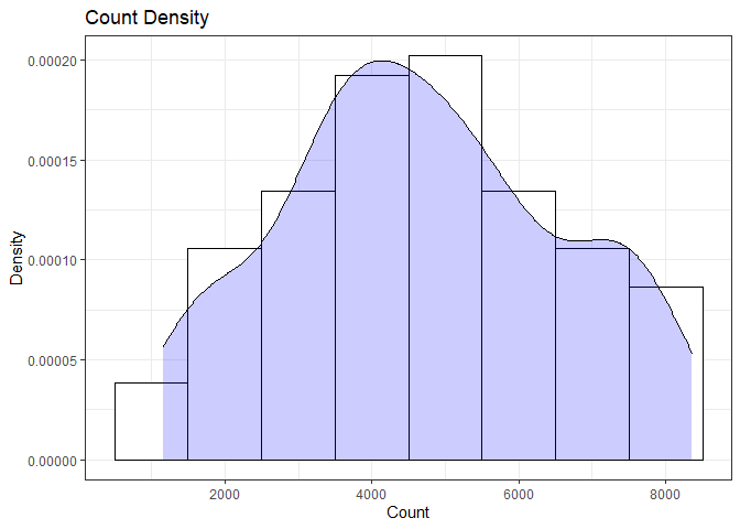
The cnt is the response variable, so we’ll use a histogram to get a
visual understanding of the variable.
ggplot(day, aes(x = cnt)) + theme_bw() + geom_histogram(aes(y =..density..), color = "black", fill = "white", binwidth = 1000) + geom_density(alpha = 0.2, fill = "blue") + labs(title = "Count Density", x = "Count", y = "Density")
summary(day$cnt)
##    Min. 1st Qu.  Median    Mean 3rd Qu.    Max.
##    1167    3391    4602    4690    5900    8362
From the histogram and summary statistics output, it is pretty evident that the count of total rental bikes are in the sub 5000 range. We will investigate if there is a relationship between the response variable and other relevant predictor variables in the next section. Lets look at the other variables individually.
#visualize numeric predictor variables using a histogram
p1 <- ggplot(day) + geom_histogram(aes(x = temp), fill = "red", binwidth = 0.03)
p2 <- ggplot(day) + geom_histogram(aes(x = atemp), fill = "red", binwidth = 0.03)
p3 <- ggplot(day) + geom_histogram(aes(x = hum), fill = "red", binwidth = 0.025)
p4 <- ggplot(day) + geom_histogram(aes(x = windspeed), fill = "red", binwidth = 0.03)
gridExtra::grid.arrange(p1,p2,p3,p4, nrow = 2)
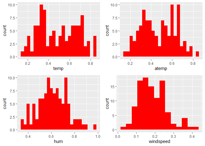
Observations:
* No clear cut pattern in tempand atemp.
-
humappears to be skewed to the left when the dataset is not filtered to a specific weekday. -
windspeedappears to be skewed(right). This variable should be transformed to curb its skewness. -
The distribution of
tempandatemplooks very similar. We should think about taking out one of the variables.
#visualize categorical predictor variables
h1 <- ggplot(day) + geom_bar(aes(x = season),fill = "pink")
h2 <- ggplot(day) + geom_bar(aes(x = yr),fill = "pink")
h3 <- ggplot(day) + geom_bar(aes(x = holiday),fill = "pink")
h4 <- ggplot(day) + geom_bar(aes(x = workingday),fill = "pink")
h5 <- ggplot(day) + geom_bar(aes(x = mnth),fill = "pink")
h6 <- ggplot(day) + geom_bar(aes(x = weathersit),fill = "pink")
gridExtra::grid.arrange(h1,h2,h3,h4,h5,h6, nrow = 3)
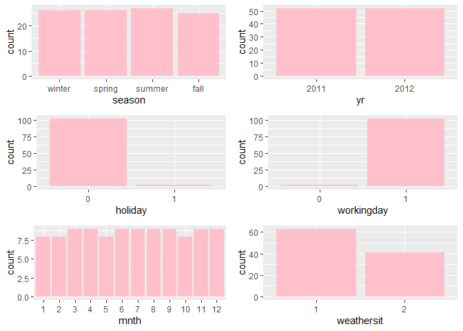
Observations:
* The variation between the four seasons is little to none.
-
About the same number of people rode bikes in 2011 and 2012.
-
Many people rode bikes on days that are not holidays.
-
Most people used the bike-sharing system on days that were neither weekends nor holidays.
-
Most people used the bike sharing system on days with clear weather.
Bi-variate Analysis
In this section, we will explore the predictor variables with respect to the response variable. The objective is to discover hidden relationships between the independent and response variables and use those findings in the model building process.
# First, we will explore the relationship between the target and numerical variables.
p1 <- ggplot(day) +geom_point(aes(x = temp, y = cnt), colour = "violet") + labs(title = "Normalized Temperature vs Total Rental Bikes")
p2 <- ggplot(day) +geom_point(aes(x = atemp, y = cnt), colour = "#FF99CC") +labs(title = "Normalized Feeling Temperature vs Total Rental Bikes")
p3 <- ggplot(day) +geom_point(aes(x = hum, y = cnt), colour = "pink") + labs(title = "Normalized Humidity vs Total rental Bikes")
p4 <- ggplot(day) +geom_point(aes(x = windspeed, y = cnt), colour = "#FF66CC") +labs(title= "Normalized Windspeed vs Total rental Bikes")
gridExtra::grid.arrange(p1, p2, p3, p4, nrow = 2)
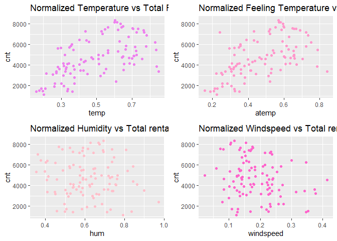
Observations:
* There appears to be a positive linear relationship between cnt ,
temp, and atemp.
- There is also a weak relationship between
cnt,hum, andwindspeed.
# Now we'll visualize the relationship between the target and categorical variables.
# Instead of using a boxplot, I will use a violin plot which is the blend of both a boxplot and density plot
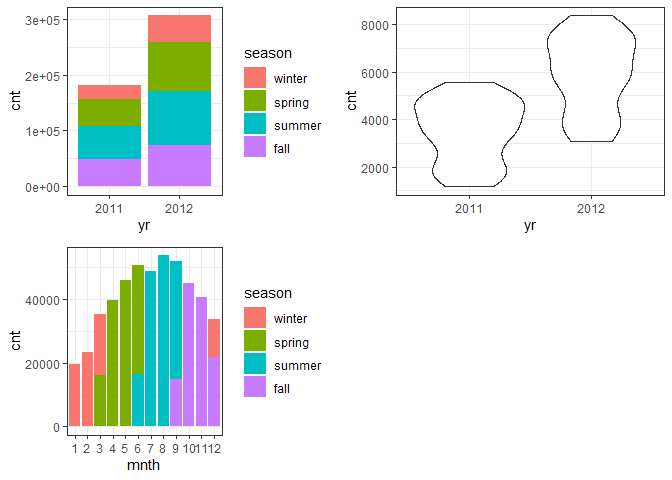
g1 <- ggplot(day) + geom_col(aes(x = yr, y = cnt, fill = season))+theme_bw()
g2 <- ggplot(day) + geom_violin(aes(x = yr, y = cnt))+theme_bw()
g3 <- ggplot(day) + geom_col(aes(x = mnth, y = cnt, fill = season))+theme_bw()
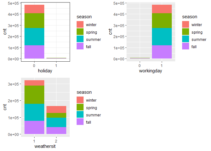
g4 <- ggplot(day) + geom_col(aes(x = holiday, y = cnt, fill = season)) + theme_bw()
g6 <- ggplot(day) + geom_col(aes(x = workingday, y = cnt, fill = season))
g7 <- ggplot(day) + geom_col(aes(x = weathersit, y = cnt, fill = season))
gridExtra::grid.arrange(g1, g2, g3, nrow = 2)
gridExtra::grid.arrange(g4, g6, g7, nrow = 2)
 Observations:
* The total bike rental count is higher in 2012 than 2011.
-
During workingday, the bike rental counts quite the highest compared to during no working day for different seasons.
-
During clear,partly cloudy weather, the bike rental count is highest and the second highest is during mist cloudy weather and followed by third highest during light snow and light rain weather.
-
The highest bike rental count was during the summer and lowest in the winter.
Correlation Matrix
Correlation matrix helps us to understand the linear relationship between variables.
day_c <- day[ , c(10:14)]
round(cor(day_c), 2)
##            temp atemp   hum windspeed   cnt
## temp       1.00  0.96  0.13     -0.20  0.60
## atemp      0.96  1.00  0.13     -0.24  0.57
## hum        0.13  0.13  1.00     -0.29 -0.09
## windspeed -0.20 -0.24 -0.29      1.00 -0.23
## cnt        0.60  0.57 -0.09     -0.23  1.00
From the above matrix, we can see that temp and atemp are highly
correlated. So we only need to include one of these variables in the
model to prevent multicollinearity. We will also transform the humidity
and windspeed variable.
day <- mutate(day, log_hum = log(day$hum+1))
day <- mutate(day, log_ws = log(day$windspeed + 1))

#Remove irrelevant variables
day <- select(day, -weekday,-holiday,-workingday,-dteday,-temp, -instant)
Model Building
First we split the data into train and test sets.
set.seed(23)
dayIndex<- createDataPartition(day$cnt, p = 0.7, list=FALSE)
dayTrain <- day[dayIndex, ]
dayTest <- day[-dayIndex, ]

# Build a tree-based model using loocv;
fitTree <- train(cnt~ ., data = dayTrain, method = "rpart",
              preProcess = c("center", "scale"),
              trControl = trainControl(method = "loocv", number = 10), tuneGrid = data.frame(cp = 0.01:0.10))
## Warning in nominalTrainWorkflow(x = x, y = y, wts = weights, info =
## trainInfo, : There were missing values in resampled performance measures.
# Build a boosted tree model using cv
fitBoost <- train(cnt~., data = dayTrain, method = "gbm",
              preProcess = c("center", "scale"),
              trControl = trainControl(method = "cv", number = 10),
              tuneGrid = expand.grid(n.trees=c(10,20,50,100,500,1000),shrinkage=c(0.01,0.05,0.1,0.5),n.minobsinnode =c(3,5,10),interaction.depth=c(1,5,10)))

# Adding a linear regression model part 2!
FitLinear <- train(cnt~ atemp + mnth*season, data = dayTrain, method = "lm", trControl = trainControl(method = "cv", number = 10))
## Warning in predict.lm(modelFit, newdata): prediction from a rank-deficient
## fit may be misleading

## Warning in predict.lm(modelFit, newdata): prediction from a rank-deficient
## fit may be misleading

## Warning in predict.lm(modelFit, newdata): prediction from a rank-deficient
## fit may be misleading

## Warning in predict.lm(modelFit, newdata): prediction from a rank-deficient
## fit may be misleading

## Warning in predict.lm(modelFit, newdata): prediction from a rank-deficient
## fit may be misleading

## Warning in predict.lm(modelFit, newdata): prediction from a rank-deficient
## fit may be misleading

## Warning in predict.lm(modelFit, newdata): prediction from a rank-deficient
## fit may be misleading

## Warning in predict.lm(modelFit, newdata): prediction from a rank-deficient
## fit may be misleading

## Warning in predict.lm(modelFit, newdata): prediction from a rank-deficient
## fit may be misleading

## Warning in predict.lm(modelFit, newdata): prediction from a rank-deficient
## fit may be misleading
# Display information from the tree fit
fitTree$results
##     cp     RMSE Rsquared      MAE  RMSESD RsquaredSD   MAESD
## 1 0.01 992.3839      NaN 992.3839 587.257         NA 587.257
# Display information from the boost fit
fitBoost$results
##     shrinkage interaction.depth n.minobsinnode n.trees      RMSE
## 1        0.01                 1              3      10 1836.3356
## 7        0.01                 1              5      10 1837.6232
## 13       0.01                 1             10      10 1832.9687
## 55       0.05                 1              3      10 1584.9613
## 61       0.05                 1              5      10 1593.5064
## 67       0.05                 1             10      10 1597.6202
## 109      0.10                 1              3      10 1400.8835
## 115      0.10                 1              5      10 1361.2633
## 121      0.10                 1             10      10 1384.0756
## 163      0.50                 1              3      10 1009.6140
## 169      0.50                 1              5      10  902.1467
## 175      0.50                 1             10      10 1106.9523
## 19       0.01                 5              3      10 1773.8915
## 25       0.01                 5              5      10 1781.5806
## 31       0.01                 5             10      10 1824.8012
## 73       0.05                 5              3      10 1410.4121
## 79       0.05                 5              5      10 1416.2209
## 85       0.05                 5             10      10 1559.6555
## 127      0.10                 5              3      10 1116.5147
## 133      0.10                 5              5      10 1187.8571
## 139      0.10                 5             10      10 1343.4134
## 181      0.50                 5              3      10  952.9201
## 187      0.50                 5              5      10  882.9106
## 193      0.50                 5             10      10  945.0783
## 37       0.01                10              3      10 1769.5015
## 43       0.01                10              5      10 1781.9106
## 49       0.01                10             10      10 1821.5846
## 91       0.05                10              3      10 1394.2375
## 97       0.05                10              5      10 1432.8331
## 103      0.05                10             10      10 1581.8119
## 145      0.10                10              3      10 1089.3432
## 151      0.10                10              5      10 1174.4976
## 157      0.10                10             10      10 1340.2634
## 199      0.50                10              3      10  899.5306
## 205      0.50                10              5      10  845.9158
## 211      0.50                10             10      10 1047.9013
## 2        0.01                 1              3      20 1777.0119
## 8        0.01                 1              5      20 1776.7096
## 14       0.01                 1             10      20 1771.6139
## 56       0.05                 1              3      20 1386.4412
## 62       0.05                 1              5      20 1390.7720
## 68       0.05                 1             10      20 1380.0745
## 110      0.10                 1              3      20 1168.8315
## 116      0.10                 1              5      20 1149.9091
## 122      0.10                 1             10      20 1146.4105
## 164      0.50                 1              3      20  914.6125
## 170      0.50                 1              5      20  839.1239
## 176      0.50                 1             10      20  964.3758
## 20       0.01                 5              3      20 1658.5706
## 26       0.01                 5              5      20 1675.2419
## 32       0.01                 5             10      20 1751.1232
## 74       0.05                 5              3      20 1144.9245
## 80       0.05                 5              5      20 1167.9899
## 86       0.05                 5             10      20 1336.0648
## 128      0.10                 5              3      20  906.1827
## 134      0.10                 5              5      20  925.8241
## 140      0.10                 5             10      20 1102.2651
## 182      0.50                 5              3      20 1024.9762
## 188      0.50                 5              5      20  933.7983
## 194      0.50                 5             10      20  984.3598
## 38       0.01                10              3      20 1661.1338
## 44       0.01                10              5      20 1672.0303
## 50       0.01                10             10      20 1750.6795
## 92       0.05                10              3      20 1108.4241
## 98       0.05                10              5      20 1166.6409
## 104      0.05                10             10      20 1339.6171
## 146      0.10                10              3      20  876.5939
## 152      0.10                10              5      20  962.4768
## 158      0.10                10             10      20 1105.1581
## 200      0.50                10              3      20  931.4003
## 206      0.50                10              5      20  840.0720
## 212      0.50                10             10      20 1023.5954
## 3        0.01                 1              3      50 1607.5856
## 9        0.01                 1              5      50 1606.2644
## 15       0.01                 1             10      50 1606.0114
## 57       0.05                 1              3      50 1079.2681
## 63       0.05                 1              5      50 1073.5991
## 69       0.05                 1             10      50 1130.7632
## 111      0.10                 1              3      50  944.7485
## 117      0.10                 1              5      50  922.9522
## 123      0.10                 1             10      50  962.5685
## 165      0.50                 1              3      50  915.8619
## 171      0.50                 1              5      50  853.6663
## 177      0.50                 1             10      50  925.6763
## 21       0.01                 5              3      50 1404.5371
## 27       0.01                 5              5      50 1422.8902
## 33       0.01                 5             10      50 1569.8138
## 75       0.05                 5              3      50  875.6778
## 81       0.05                 5              5      50  882.4982
## 87       0.05                 5             10      50 1062.6730
## 129      0.10                 5              3      50  780.7774
## 135      0.10                 5              5      50  805.2725
## 141      0.10                 5             10      50  928.0897
## 183      0.50                 5              3      50 1015.6769
## 189      0.50                 5              5      50  916.3530
## 195      0.50                 5             10      50  932.4290
## 39       0.01                10              3      50 1394.0236
## 45       0.01                10              5      50 1426.2763
## 51       0.01                10             10      50 1569.9244
## 93       0.05                10              3      50  842.4789
##      Rsquared       MAE   RMSESD RsquaredSD    MAESD
## 1   0.6087974 1512.1892 187.7934  0.2290785 198.2450
## 7   0.6080189 1515.6120 186.0200  0.2331195 197.9163
## 13  0.6138054 1510.4863 190.3715  0.2168574 200.2716
## 55  0.7181949 1311.8358 176.0739  0.1870134 184.3798
## 61  0.7358287 1318.5167 180.9814  0.1708065 187.1937
## 67  0.6560545 1320.6680 178.8415  0.1889993 197.0915
## 109 0.7091520 1150.1569 147.6370  0.1738678 179.3422
## 115 0.7415625 1126.3995 169.3279  0.1648559 191.5234
## 121 0.7154709 1135.0674 166.2747  0.1651167 196.0373
## 163 0.7475498  857.8479 279.8473  0.1828965 259.0340
## 169 0.7915612  770.1874 258.0004  0.1460511 236.5353
## 175 0.6996485  941.6772 314.9833  0.2044293 244.7280
## 19  0.7528079 1461.0915 181.2850  0.1574667 189.5808
## 25  0.7307300 1470.3681 176.3829  0.1858863 184.6933
## 31  0.6034857 1499.7166 187.9904  0.2205980 197.8606
## 73  0.7742331 1173.2207 142.9792  0.1571939 142.5942
## 79  0.7468056 1185.3641 160.4969  0.1542639 175.7797
## 85  0.6814140 1302.5248 173.8763  0.2208641 186.8790
## 127 0.7879140  952.0725 133.0506  0.1413387 132.0469
## 133 0.7530893  997.1658 168.6068  0.1655733 176.9052
## 139 0.6851757 1131.9358 178.4248  0.1674030 200.5332
## 181 0.7639558  782.1383 321.7371  0.1619225 248.5019
## 187 0.8140124  727.7466 200.2336  0.0927589 156.6424
## 193 0.7703283  759.1065 193.1422  0.1432561 160.2380
## 37  0.7635976 1458.1661 178.0948  0.1262080 187.6886
## 43  0.7407987 1463.5030 184.6442  0.1763252 190.3307
## 49  0.6556054 1498.6920 189.0027  0.1861643 199.9607
## 91  0.7580407 1173.8759 131.1466  0.1611976 136.4853
## 97  0.7495401 1194.3097 158.3852  0.1309655 162.0060
## 103 0.6839635 1318.3319 171.8847  0.2053783 187.4353
## 145 0.8015008  914.9764 173.3996  0.1275347 183.0272
## 151 0.7588779  979.8749 179.7136  0.1430890 193.5920
## 157 0.7391377 1122.0462 181.7407  0.1635621 203.1259
## 199 0.7812466  735.1251 303.8354  0.1539557 216.7674
## 205 0.7970255  703.9597 295.6545  0.1861333 226.1972
## 211 0.7031801  888.5490 244.8979  0.1738567 201.4794
## 2   0.6270996 1468.9936 182.1041  0.2362285 190.0238
## 8   0.6383654 1471.3739 182.2205  0.2338646 188.3023
## 14  0.6422747 1463.8914 187.9827  0.2042563 197.5553
## 56  0.7372061 1144.8434 177.5049  0.1717411 187.7444
## 62  0.7290280 1147.2433 158.7730  0.1809952 170.5596
## 68  0.7204127 1147.2179 168.7043  0.1587271 189.8160
## 110 0.7436299  999.2881 169.9058  0.1751260 189.2480
## 116 0.7544253  969.2710 187.2565  0.1701369 193.2927
## 122 0.7514357  986.8911 191.9062  0.1807015 195.1423
## 164 0.7853151  731.7926 216.9089  0.1318945 198.0447
## 170 0.8151544  688.7626 289.3370  0.1660283 222.9503
## 176 0.7557424  823.6524 274.1686  0.1664357 229.2051
## 20  0.7639873 1370.9669 167.0685  0.1588590 171.9050
## 26  0.7432804 1385.3523 166.2781  0.1766339 171.6862
## 32  0.6876977 1442.1157 181.3777  0.1806353 187.1353
## 74  0.7908635  965.5197 140.9580  0.1433702 152.4958
## 80  0.7749532  992.1783 145.8718  0.1517034 183.3191
## 86  0.7180776 1129.2794 175.1463  0.1799555 206.6252
## 128 0.8009733  791.6819 197.9517  0.1384365 185.0792
## 134 0.8020368  792.3637 187.7212  0.1321687 156.7176
## 140 0.7296594  973.8703 205.7767  0.1416052 189.5624
## 182 0.7401692  825.5650 308.9536  0.1523572 224.7369
## 188 0.7796155  763.8488 253.1871  0.1170723 208.1129
## 194 0.7495737  792.4166 221.6888  0.1418188 179.9189
## 38  0.7774801 1372.6090 160.6476  0.1511904 166.0353
## 44  0.7831074 1377.0422 176.4546  0.1438892 179.2032
## 50  0.6863917 1444.5806 183.8881  0.1834599 189.0605
## 92  0.7980700  930.4894 148.2904  0.1601672 165.4853
## 98  0.7691855  978.2375 167.2653  0.1383647 167.7809
## 104 0.7387034 1118.0501 157.7567  0.1744582 181.2332
## 146 0.8203214  744.1093 222.4728  0.1106965 186.2892
## 152 0.7879228  824.2471 189.6248  0.1365617 165.4878
## 158 0.7486989  978.0923 202.8069  0.1682499 196.0673
## 200 0.7646082  758.5337 309.0609  0.1512862 229.7256
## 206 0.8194823  723.8848 278.4732  0.1466171 229.8137
## 212 0.7194507  861.6289 247.2595  0.1870449 212.2485
## 3   0.7079203 1330.3399 169.1017  0.1685300 174.7901
## 9   0.7065198 1329.7362 171.5230  0.1812985 176.9566
## 15  0.6882842 1333.3966 174.9430  0.1727206 184.6150
## 57  0.7723610  923.2522 208.7081  0.1583586 223.4222
## 63  0.7674799  931.0982 200.6594  0.1611581 204.3842
## 69  0.7169191  995.0249 189.3940  0.1577650 197.8794
## 111 0.7934828  800.7096 231.1513  0.1528192 222.9414
## 117 0.7963591  796.5328 249.3491  0.1624429 236.3055
## 123 0.7684146  848.7784 261.9339  0.1745838 236.9628
## 165 0.7965826  735.3046 270.9326  0.1593465 263.0521
## 171 0.8056713  693.2902 301.5266  0.1597299 218.9540
## 177 0.7637095  765.1737 250.2241  0.1658553 198.9043
## 21  0.7790224 1170.2558 141.3031  0.1541726 153.6129
## 27  0.7600093 1183.7976 146.7062  0.1686291 163.9674
## 33  0.7093251 1298.0809 178.2260  0.1727116 184.4827
## 75  0.8172655  742.1908 203.4804  0.1375519 175.1933
## 81  0.8076912  760.1537 236.9006  0.1526785 211.6746
## 87  0.7416104  942.1328 213.3260  0.1585077 190.8857
## 129 0.8354204  644.7805 239.0794  0.1215048 174.6346
## 135 0.8267100  673.4790 223.3460  0.1218087 197.7691
## 141 0.7737822  811.8741 244.6512  0.1390676 229.9847
## 183 0.7447637  840.3558 327.6790  0.1477981 262.1112
## 189 0.7801213  761.2207 297.8166  0.1294020 246.1949
## 195 0.7635566  755.2140 192.6836  0.1292737 155.1552
## 39  0.7899369 1166.1104 134.8837  0.1471150 145.7362
## 45  0.7707516 1186.8266 154.4815  0.1616002 163.9083
## 51  0.6977832 1299.1601 180.6022  0.1624456 186.7607
## 93  0.8236717  714.9868 203.4771  0.1307451 164.5665
##  [ reached 'max' / getOption("max.print") -- omitted 116 rows ]
# Display information from the linear model fit
FitLinear$results
##   intercept     RMSE  Rsquared      MAE   RMSESD RsquaredSD    MAESD
## 1      TRUE 1725.682 0.3255188 1502.304 448.4066  0.2626169 413.9164
Now, we make predictions on the test data sets using the best model fits. Then we compare RMSE to determine the best model.
predTree <- predict(fitTree, newdata = select(dayTest, -cnt))
postResample(predTree, dayTest$cnt)
##         RMSE     Rsquared          MAE
## 1162.5705442    0.5827969  961.7493718
boostPred <- predict(fitBoost, newdata = select(dayTest, -cnt))
postResample(boostPred, dayTest$cnt)
##         RMSE     Rsquared          MAE
## 1132.3827792    0.6092506  791.1667375
linearPred <- predict(FitLinear, newdata = select(dayTest, -cnt))
## Warning in predict.lm(modelFit, newdata): prediction from a rank-deficient
## fit may be misleading
postResample(linearPred, dayTest$cnt)
##        RMSE    Rsquared         MAE
## 1680.147374    0.229037 1330.801141
When we compare the two models, the boosted tree model has lower RMSE values when applied on the test dataset. Hence, the boosted tree model is our final model and best model for interpreting the bike rental count on a daily basis.